The eigensystem of the Gaussian kernel w.r.t. a Gaussian measure
This blogpost composed in collaboration with Yuxi Liu, who did much of the analytical legwork.
A large number of recent works have converged on the conclusion that the behavior and performance of kernel methods (and kernel regression in particular) can be simply described in terms of the eigenstructure of the task with respect to the kernel. To restate: we can understand kernel regression to the degree we understand the eigenstructure of the task.
It is generally not too hard to diagonalize the kernel and obtain the task eigenstructure numerically, and this has lead to a great deal of insight into the learning behavior of kernel regression. However, it’s generally quite difficult to find task eigenstructure analytically, even in simple toy cases, as it usually requires computing some complicated integrals. As every physicist knows, there are major advantages to analytical solutions: insight and intuition are often more easily extracted from symbolic solutions, and by taking limits a single analytical solution can give a system’s phenomenology in several different regimes. It thus behooves us to collect analytically solvable cases and sit with them to extract generalizing intuition. To that end, in this blogpost, we will give the analytical eigenstructure for the Gaussian kernel on a 1D Gaussian distribution.
What exactly diagonalizable cases are known?
The first cases one turns to when one wants an exact analytical eigensystem are settings where the kernel and the domain share a symmetry. For example, with a translation-invariant kernel on a translation-invariant domain (e.g. the $d$-torus) or a rotation-invariant kernel on a rotation-invariant-domain (e.g. the $d$-sphere), the eigenfunctions are simply the harmonic functions on the domain (plane waves or spherical harmonics in the two named cases), and the eigenvalues are given by the Fourier transform of the kernel. Some high-dimensional problems resemble these cases when the number of dimensions goes to infinity (e.g. Mei + Montanari (2019)).
Solvable finite-dimensional cases without exact symmetry are rare. It seems worth considering such cases, since real data rarely has such symmetry, and the eigenfunctions are only nontrivial if there’s no exact symmetry. Zhu et al. (1997) treat a very similar case to the one we develop here. I don’t really know any other examples of exactly solvable cases. If you know any more, let me know. It seems worth compiling a list!
Problem setup: Gaussian kernel on a 1D Gaussian distribution
Consider a scalar normal random variable $x \sim \mathcal{N}(0,\sigma^2)$, where $\sigma^2$ is the variance of the distribution. Consider learning on this distribution with a Gaussian kernel
\[K(x,y)=e^{-\frac{(x-y)^2}{2 w^2}}\]where $w$ is the width of the kernel. We seek an eigendecomposition
\[K(x,y) = \sum_k \lambda_k \, \phi_k(x) \, \phi_k(y),\]where $\lbrace \lambda_k \rbrace$ are nonnegative eigenvalues and $\lbrace \phi_k \rbrace$ are eigenfunctions satisfying the orthonormality relation
\[\mathbb{E}_x[\phi_k(x) \phi_\ell(x)] = \delta_{k\ell}.\]We refer to $\lbrace \lambda_k \rbrace$ and $\lbrace \phi_k \rbrace$ together as the kernel eigensystem or eigenstructure.
Main result: analytical form of the eigenstructure
Hermite polynomials
Let $h_k(x) \equiv \frac{1}{\sqrt{k!}} \text{He}_k(x)$ denote the (rescaled) probabilist’s Hermite polynomials. The normalization prefactor $\frac{1}{\sqrt{k!}}$ is chosen so that $\mathbb{E}_{x \sim \mathcal{N}(0,1)}[h_k^2(x)] = 1$.
The eigenstructure in closed form
Note that the eigenfunctions resemble the eigenfunctions of the quantum harmonic oscillator but with different scale factors $\alpha \neq\beta$ on the exponential and Hermite components. The eigenvalues are a geometric series with ratio $r < 1$.
Obtaining the answer
We obtained these eigenfunctions treating Equations 1,2 as an ansatz and solving for $\alpha, \beta, c, r$. This is doable with Mehler’s formula and algebraic manipulation. Here is a step-by-step derivation.
Visualizing the eigenstructure
We can plot the eigenfunctions and eigenvalues and compare analytical formulae with numerics to make sure we’re right. Here’s a colab notebook that does so, and here’s the resulting plot:
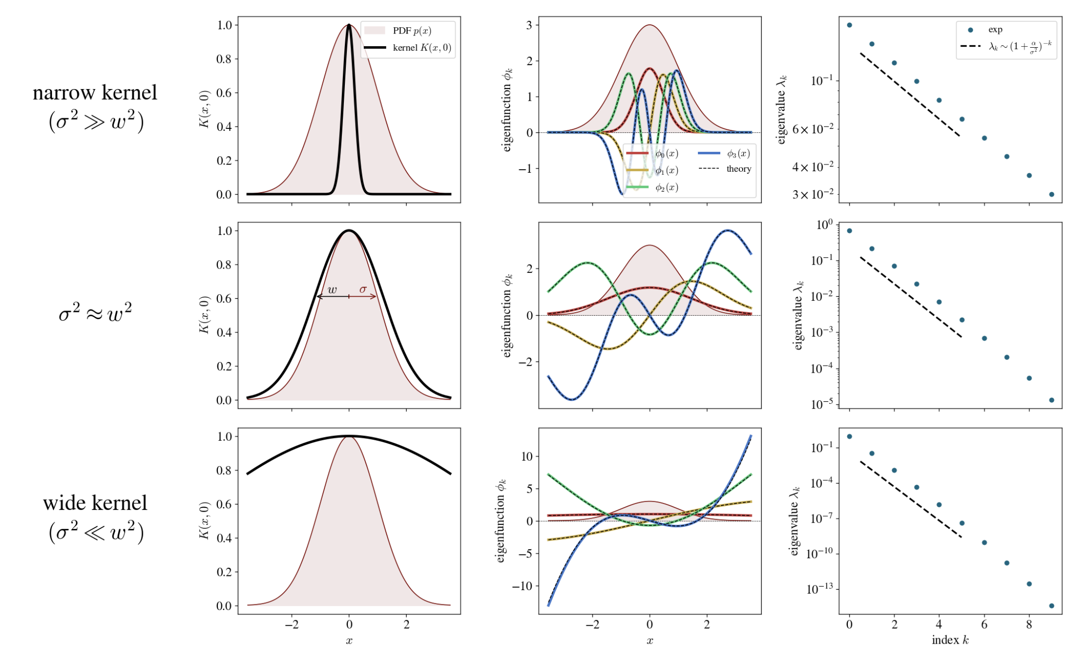
Each row shows the eigenstructure for a different ratio $\frac{w^2}{\sigma^2}$. The leftmost plot in each row is a simple visualization of the Gaussian PDF (which here always has $\sigma^2 = 1$) and the Gaussian kernel. The middle plot in each row shows the first five kernel eigenfunctions with theoretical curves overlaid for comparison. The rightmost plot in each row shows the kernel eigenvalues. We find that the experimental eigenvalues indeed follow the predicted geometric descent (with small deflections due to numerical error).
Eigenstructure in two limits
Looking at the top and bottow rows in the above figure, we get the feeling it might be informative to examine the $\sigma^2 \gg w^2$ and $\sigma^2 \ll w^2$ limits of our analytical expressions. Here’s what you get:
Narrow kernel: $\sigma^2 \gg w^2$
\[\begin{aligned} \alpha &\approx \sqrt{\sigma w}, \\[6pt] \beta &\approx \sqrt{\frac{\sigma w}{2}}, \\[6pt] c &\approx \left( \frac{2 \sigma}{w} \right)^{1/4}, \\[6pt] r &\approx 1. \end{aligned}\]In this regime, the scale factors $\alpha, \beta$ are the same up to a factor of $\sqrt{2}$, and the resulting eigenfunctions $\phi_k$ are exactly the eigenfunctions of the quantum harmonic oscillator (note that we’re using probabilist’s instead of physicist’s Hermite polynomials). This makes sense, as we’d expect the eigenfunctions of a sufficiently narrow Gaussian kernel to converge to the eigenfunctions of the Laplacian. The ratio $r = \frac{\lambda_{k+1}}{\lambda_k}$ approaches $1$, which tells us that the top eigenfunctions have practically identical eigenvalues.
Wide kernel: $\sigma^2 \ll w^2$
\[\begin{aligned} \alpha &\approx w, \\[6pt] \beta &\approx \sigma, \\[6pt] c &\approx 1, \\[6pt] r &\approx \frac{\sigma^2}{w^2}. \end{aligned}\]This is the more interesting regime. In this case, $\alpha$ and $\beta$ decouple, and in fact $\alpha \approx w \gg \sigma$ is so wide that the exponential factor in the functional form of $\phi_k(x)$ becomes irrelevant, and we’re left with just a Hermite polynomial. You can see this in the bottom row of the figure above: the eigenfunctions start to just look like polynomials of increasing order. The eigenvalue ratio $r \approx \frac{\sigma^2}{w^2}$ approaches the ratio of the distribution variance to the kernel variance. These two facts are the main things I wanted to get out of this calculation.
How “Hermite” are the eigenfunctions for varying values of $\sigma^2 / w^2$?
Let us perform a numerical experiment: we shall compute the true kernel eigenfunctions ${\phi_k}$, compute the Hermite polynomials ${h_k}$, and for each $k$, find the cosine similarity \(\frac{\langle \phi_k, h_k \rangle}{\| h_k \|}\) where the inner product \(\langle f, g \rangle = \mathbb{E}_x[f(x) g(x)]\) is the $L^2$ inner product w.r.t. the measure.
The results are plotted below:
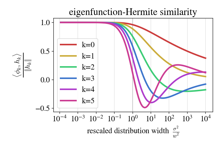
A few observations:
- at larger $k$, we require smaller $\gamma \equiv \frac{\sigma^2}{w^2}$ to approach Hermiteness, and
- $\gamma < 0.1$ is generally small enough, at least up to $k = 3$ or $4$.
Implications and next steps
The main takeaway here is that so long as $\sigma^2$ is sufficiently smaller than $w^2$ — and we don’t care exactly how small — the kernel’s “eigenfeatures” are simply the “Hermite features” of the data. In this regime, the kernel eigenvalues are simply powers of $\frac{\sigma^2}{w^2}$. Nice!
What’s next? It’s likely that a more general class of kernels (including in higher dimension) can be solved using these techniques, and if that’s the case, it’s worth compiling these exactly solvable cases and extracting what intuition we can. Even with this 1D Gaussian case, though, there are probably ways to take this result and apply its intuition to kernel learning problems on (potentially realistic) high-dimensional data.