It's hard to turn a low-rank matrix into a high-rank matrix

In this blogpost, I point out that applying a nonlinear function to a low-rank random matrix cannot make it into a high-rank matrix.

Large random matrices can often be profitably understood in terms of their singular value spectrum. One useful distinction is between high (effective) rank and low (effective) rank matrices. Low-rank matrix effects are important in deep learning, and if you listen to the whispers of deep learning theorists, they’re cropping up on the margins everywhere. My money’s on their assuming a central role in our understanding of deep learning in the coming years.

This blogpost conveys a particular idea about low-rank matrices: it’s really hard to deterministically transform them into high-rank matrices. It’s written mostly for myself, but hopefully it’s useful to others.

Trying and failing to turn a low-rank matrix high-rank

Suppose we independently sample two random vectors $\mathbf{x}, \mathbf{y} \sim \mathcal{N}(\mathbf{0}, \mathbf{I}_n)$ with dimension $n$ and standard Gaussian entries. From these vectors, we can construct the rank-one matrix $\mathbf{A} = \frac{1}{n} \mathbf{x}\mathbf{y}^\top$. The matrix $\mathbf{A}$ will have one nonzero singular value with value approaching $\sigma_1 = 1$ as $n$ grows.

Suppose we want to turn this low-rank matrix into a high-rank matrix, with many singular values of the same order as the largest. Suppose we must accomplish this via some simple transformation, but we have no access to additional randomness, so it’s got to be a deterministic function. The most basic thing we might try is to choose some nonlinear function $\phi: \mathbb{R} \rightarrow \mathbb{R}$ and apply it elementwise to each matrix entry to get $\mathbf{A}_\phi = \frac{1}{n} \phi \circ (\mathbf{x}\mathbf{y}^\top)$.

This seems promising! Having rank one is a very fragile condition, and so we expect that almost any such nonlinearity would break that condition and give us a matrix with a singular spectrum more like that of a full-rank matrix.

Well, let’s try it. Here are some examples:

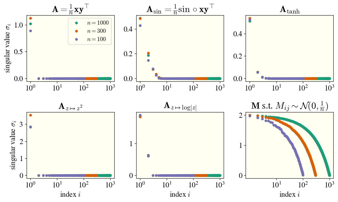
In the top left plot, I’ve shown the singular spectrum of a rank-one matrix for three values of $n$. In the next four plots, I show the singular spectrum of matrices $\mathbf{A}_\phi$ for various $\phi$. In the final plot, I show the spectrum of a full-rank random matrix with i.i.d. entries, again for various $n$.

What’s happened? None of the matrices $\mathbf{A}_\phi$ are still rank-one (well, except for $\phi: z \mapsto z^2$), but they seem to only have a handful of singular values of order unity. (They’re actually all nonzero, but they decay really fast.) Their spectra don’t look anything like the singular spectra of the full-rank matrix, which for large $n$ have many eigenvalues close to $\sigma_1$.

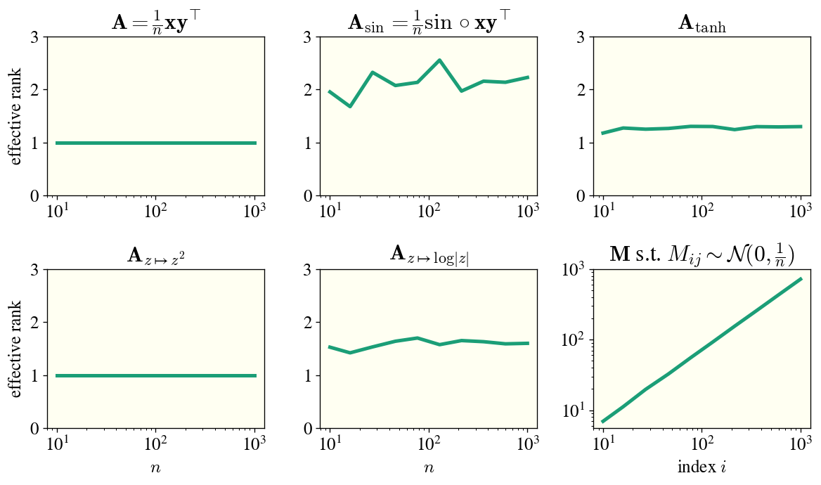
One way to characterize this difference is through the effective rank of the matrix, defined for a matrix $\mathbf{M}$ as $\text{erank}(\mathbf{M}) = \frac{(\sum_i \sigma_i(\mathbf{M}))^2}{\sum_i \sigma_i^2(\mathbf{M})}$. Here I will plot the effective rank of these same matrices as $n$ increases:

We see clearly that the effective rank quickly stabilizes at an order-unity value in each case, while the effective rank of a dense random matrix grows proportionally to $n$. What’s going on?

The explanation: constructing the singular spectrum

We will now explain what’s going on. Remarkably, we can understand this by explicitly constructing the singular vectors for large $n$.

Warmup: the square function

We’ll start with the case of the square function, which seems like the easiest. For ease of explanation, let’s give it the notation $\xi: z \mapsto z^2$.

The left- and right- singular vectors of $\mathbf{A} = \frac{1}{n} \mathbf{x}\mathbf{y}^\top$ are (proportional to) $\mathbf{x}$ and $\mathbf{y}$, respectively. What about the matrix $\mathbf{A}_\xi = \frac{1}{n} \xi \circ \mathbf{x}\mathbf{y}^\top$? Well, this matrix has entries $A_{\xi;i,j} = \frac{1}{n} x_i^2 y_j^2$, from which we can see that

\[\mathbf{A}_\xi = \frac{1}{n} \left( \xi \circ \mathbf{x} \right)\left( \xi \circ \mathbf{y} \right)^\top.\]

That is, because $\xi$ has the special property that $\xi(ab) = \xi(a) \cdot \xi(b)$, the resulting matrix $\mathbf{A}_\xi$ is actually still rank-one, and its singular vectors are pointwise-nonlinearly transformed versions of the originals. This is also true for many other common functions, including $\phi \in {\mathrm{sign}, \mathrm{abs}}$ and indeed any monomial. It’s worth noting that the condition for preserving rank-one-ness is actually just that $\xi(ab) = f(a) \cdot g(b)$ for some functions $f, g$; these functions need not equal $\xi$.

The general case

To get the case of general $\phi$, we’ll actually consider an even larger set of matrices: matrices $\mathbf{H}$ such that $H_{ij} = \frac{1}{n} h(x_i, y_j)$ for a bivariate function $h : \mathbb{R} \times \mathbb{R} \rightarrow \mathbb{R}$. The difference is that we’re not requiring this function to have the form $h(xy)$; it can be an arbitrary bivariate function.

We now have a function $h(x, y)$ and probability measures $\mu_x, \mu_y$ from which $x, y$ can each be sampled (namely, both $\mu_x, \mu_y$ are unit Gaussian). This means that we can define what I think of as the “operator SVD” of the function $h$, which means writing it in the form

\[h(x, y) = \sum_i \sigma_i f_i(x) g_i(y),\]

where ${ \sigma_i }$ are nonnegative singular values indexed in nonincreasing order and the functions ${f_i}, {g_i}$ are orthonormal bases in the sense that $\mathbb{E}_{x \sim \mu_x} [f_i(x) f_j(x)] = \delta_{ij}$ and $\mathbb{E}_{y \sim \mu_y} [g_i(x) g_j(x)] = \delta_{ij}$.¹

The upshot is that the first singular value of $\mathbf{A}_\phi$ will be approximately the value $\sigma_1$ obtained from the operator SVD of $h(x, y) = \phi(xy)$, and the first singular vectors are going to be approximately $f_1(\mathbf{x})$ and $g_1(\mathbf{y})$. Ditto with the second and third and so on. These generally decay fairly fast (faster than a powerlaw if $h$ is analytic, I believe), so in the examples above, you usually end up with only a handful of singular values appreciably above zero. Because this spectrum is asympotically independent of the matrix size $n$ (which merely determines the error to which one approximates it), we have order-unity effective rank. Deterministic nonlinear functions applied elementwise can’t bring a matrix from rank one to full rank!

As an aside, I don’t actually know how to compute the operator SVD of a generic $h$ analytically. I’d guess there’s no general form, even for Gaussian $\mu_x, \mu_y$. However, we could approximate it numerically by taking some finite-size sample of $x, y$ and working from that, and in fact, computing the singular values of $\mathbf{A}_\phi$ is precisely computing a Monte Carlo estimate of the operator singular spectrum of $h$, and ditto for the singular vectors.

An even more general case: rank-$k$ inputs

Well, what if instead of our original matrix isn’t the rank-one matrix $\frac{1}{n} \mathbf{x} \mathbf{y}^\top$ but instead the rank-$k$ matrix $\frac{1}{n} \mathbf{X} \mathbf{Y}^\top$, with $\mathbf{X}, \mathbf{Y} \in \mathbb{R}^{n \times k}$ having standard Gaussian entries and $k = O_n(1)$? Well, turns out that’s fine — you can do the same argument as above, but instead of a scalar bivariate function $h(x, y)$, you end up having to consider a function of two $k$-dimensional vectors $h(\mathbf{\bar{x}}, \mathbf{\bar{y}})$, where $\mathbf{\bar{x}}, \mathbf{\bar{y}}$ represent rows of $\mathbf{X}, \mathbf{Y}$, respectively. (To see this, note that the matrix entries look like $\phi(\mathbf{\bar{x}}^\top \mathbf{\bar{y}})$, and then we’re taking a generalization like we did before.) You can then compute the operator SVD in the same way, where now e.g. $f_i : \mathbb{R}^{k} \rightarrow \mathbb{R}$ are functions of vectors, not scalars. The rest of the argument goes through the same way. This can also be extended to different types of nonlinear functions: for example, if instead of acting elementwise, $\phi$ acts jointly on $k \times k$ submatrices, this still carries through. I’d guess that basically any matrix transformation which acts locally, is blind to the global index of a local region, and is smooth will admit basically the same argument.

Relevance to deep learning

One reason this stuff matters is that gradient updates to matrices are low-rank, but modern optimizers (Adam, SignSGD, etc.) often don’t update in the true direction of the gradient, instead applying some kind of elementwise preconditioning. This story about the robustness of low-rankness means that even with these modern optimizers, we expect this low-rank behavior to remain pretty strongly in effect regardless of the optimizer. This is basically why conclusions about the scaling behavior for SGD at infinite width continue to apply (with appropriate modification) for Adam and other optimizers even though their updates aren’t gradient-aligned.

Some questions I still have

• Can this be understood via some kind of “entropy” argument? It’d be very cool if something like the following could be made rigorous: we only had a $\Theta(n)$ “amount of randomness” to begin with, but a full-rank random matrix has an “amount of randomness” scaling as $\Theta(n^2)$, so we couldn’t possibly close that gap with a deterministic function, and we need another source of randomness to do so.
• What if the rank $k$ isn’t order-unity, but it’s also not order-$n$, but instead scales like say $k \sim n^{1/2}$? Does the effective rank remain $O(k)$? Seems likely.

---

Thanks to Greg Yang for pointing this out to me during the development of this paper.

---