Time-reversed random walks

A year or so ago, at the height of the pandemic, a few friends and I watched Tenet (2020), an action movie whose core conceit is that certain people and objects move the opposite direction through time. The idea’s not that they time-travel or that they merely age backwards, it’s that they’re truly time-reversed, appearing to ordinary observers like a video played backwards. To get an idea of what I mean, here’s a clip of the protagonists fighting two time-reversed opponents.

Does this concept make sense? Thinking about it for a bit, one immediately bumps up against a number of free-will-related paradoxes. For example, if you start a fight with a time-reversed adversary, it seems you’re guaranteed you won’t incapacitate them because you observed them up and fighting at a time that’s earlier for you but later for them (if you are to win, you must have “recapactitated” them with your first blow). Similarly, it seems you couldn’t break a time-reversed vase or light a time-reversed match, and things would probably end badly if you tried to eat a time-reversed sandwich. Ultimately, however, these are paradoxes of human agency, and if you remove free will as a consideration, these events’ impossibility feels more believable. Accepting the lack of free will, is the movie’s core idea physically possible?

At a first glance, it looks like several scenes clearly violate Newtonian mechanics, such as this scene in which a gear jumps off a table to meet a hand that dropped it backwards in time. However, it turns out this is not strictly impossible: the thermally jiggling particles of the surface beneath the gear could all come together and move in the same direction, giving the gear a big push upwards and leaving the surface a little colder. This is precisely the time-reversed process of the forwards event of dropping the gear. This sequence of steps seems absurdly implausible - and in our world, it would be - but it doesn’t break conservation of momentum or energy or violate any ironclad law of physics. These sorts of backwards processes are always possible because the laws of Newtonian physics and electromagnetism are time-reversal symmetric¹.

It turns out the apparent flow of time in the world we see around us is due principally to thermodynamics, a statistical set of effective laws that emerge from the basic rules of the universe when considering macroscopic systems like vases and Christopher Nolan. Time-reversed versions of events are not fundamentally impossible even in ordinary circunstances, they’re merely much less likely than their forwards-time counterparts. In practice, the gear will stay on the surface for as long as you watch it, but there is indeed a miniscule probability it’ll jump up to meet your hand each moment. In a very deep sense, fragile objects shatter forwards in time because, well, they’re not broken now, and there are lots of ways they can break, so statistics doesn’t have to work too hard to make it happen. If you sweep together a bunch of glass shards, however, there’s only one way they can all fit together, so their perfect coalescence is very unlikely. In our universe, things happen to generally be more ordered back in the direction we call the past on account of the Big Bang. However, if you took another universe and enforced the constraint that things are ordered and nice at some final time, time-reversal would give you a universe flowing “backwards” in time, though its inhabitants would of course never know the difference. This is the difference between specifying the initial and final conditions of a dynamical process, and this is no difference at all for a time-symmetric process.

Okay, but how do you get things moving both forwards and backwards? This is weird, since you normally can’t specify both initial and final conditions for a dynamical process. However, one way to do it and avoid a paradox might be to specify only partial information at both points in time. For example, suppose I enforce that the left half of a room contains person A at time \(t=0\), and the right half of the same room contains person B at time \(t=T\), and I don’t specify anything else. This is an underdetermined system which is likely to have many solutions. Actually finding one would be hard - you’d probably have to iterate forwards and backwards in time for a bunch of cycles in a nonlocal fashion until you satisfy all the boundary conditions - but it’s not impossible in principle. Given appropriate brain states in these boundary conditions, the obtained dynamical solution might be these two people fighting. This way of thinking about the problem is weird and nonlocal, but so is Tenet, and it feels more satisfying to me than prioritizing one time direction and viewing time-reversed events like the leap of the gear as simply a series of flukes.

This is a concrete enough way of looking at the problem that we could start to think about how to simulate it. The ultimate dream here would be a video game in which you fight and interact with creatures moving backwards in time. In order to make that happen, though, we need to understand how to model rule-based processes from the point of view of an observer moving the other way in time. The rest of this post obtains the math for doing this using the simplest dynamical model in thermodynamics, the random walk.

The 1D discrete random walk

The random walk is a basic stochastic process in which a particle, which we refer to as a walker, explores a space by taking steps in random directions. This process is used to model a swath of phenomena including the paths of diffusing particles, fluctuating stock prices, and the movements of foraging animals, and it’s found use in essentially every discipline of science.

The simplest example of this process is a 1D random walk with discrete steps. Let \(x_0, x_1, x_2, ..., x_t, ...\) be integers denoting the position of a random walker on the real line at each timestep. The initial condition and transition dynamics are

\[x_0 = 0,\] \[\begin{equation} \label{eqn:forward_step} x_{t+1} = \left\{ \begin{array}{lr} x_t, & p = \frac{1}{2} \\ x_t + 1, & p = \frac{1}{2}. \end{array} \right. \end{equation}\]

In words, the random walker begins at zero and, at each timestep, flips a coin and either remains put or moves to \(x \rightarrow x + 1\) accordingly. (It’s worth noting that we could’ve also chosen the possible steps to be not \(\{0,1\}\) but rather \(\{-1,1\}\) to ensure that the random walk has mean zero. It will prove mathematically simpler to use our current formulation, but we can always recover the latter setting by constructing \(\tilde{x}_t \equiv 2 x_t - t\). We will use \(\tilde{x}_t\) in our visualizations below, and we will refer to the two possible steps as “leftwards” and “rightwards.”)

Suppose we want to know \(p(x_t)\), the probability of the walker being at position \(x_t\) at time \(t\). By placing this random walk on Pascal’s triangle, it’s easy to show that this distribution is given by

\[\begin{equation} \label{eqn:p_forwards} p(x_t) = 2^{-t} \left( \begin{array}{c} t \\ x_t \end{array} \right). \end{equation}\]

Figure 1 gives an schematic illustration of this random walk as well as a visualization of many simulated runs².

                              

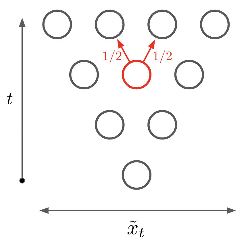
Figure 1. Left: in the 1D discrete random walk, the walker moves left or right at each timestep with probability $1/2$. Right: simulated random walks. The upper plot shows a histogram of final positions (blue) and the theoretical distribution (red).

Reversing time

The above random walks start at the origin at \(t=0\) and take uncorrelated steps from then on. This is easy to simulate, as every step is independent of every other step. Let us now imagine how these trajectories look to an observer moving backwards in time. The walkers start in a wide distribution, take fairly random steps, but then all converge at the origin at \(t=0\). Suppose you wish to find the statistics of this process from the point of view of this backwards observer: given that they observe a walker at position \(x_t\) at time \(t\), what are its transition probabilities for the step to time \(t - 1\)? (Equivalently, we could forget about the time reversal and ask about the statistics of a path conditioned on its intersecting \((t, x_t)\), but that’s less fun.)

We would like to obtain an update equation similar to Equation \(\ref{eqn:forward_step}\) which gives us the statistics of \(x_{t-1}\) as a function of \(x_t\) (because the random walk is a Markov process, we need not consider \(x_{t+1}\) and so on in finding the statistics of \(x_{t-1}\)). We can do so using Bayes’ rule, which, applied to our case, tells us that

\[p \left( x_{t-1} | x_{t} \right) = \frac{ p \left( x_{t} | x_{t-1} \right) p \left( x_{t} \right) }{ p \left( x_{t-1}\right) }.\]

Equation \(\ref{eqn:forward_step}\) gives \(p \left( x_{t} | x_{t-1} \right)\) and Equation \(\ref{eqn:p_forwards}\) tells us \(p(x_{t-1})\) and \(p(x_t)\). Inserting the results and simplifying algebraically, we find that

\[\begin{equation} \label{eqn:backward_step} x_{t-1} = \left\{ \begin{array}{lr} x_{t} - 1, & p = \frac{x_t}{t} \\ x_{t}, & p = \frac{t - x_t}{t}. \end{array} \right. \end{equation}\]

The resulting backward process is illustrated schematically in the left subfigure of Figure 2. Examining these transition probabilities, we see that, when run backwards in time, our random walk is biased towards taking a step right if \(x_t < \frac{t}{2}\) and biased towards taking a step left if \(x_t > \frac{t}{2}\), and that the probability of a step left interpolates linearly from \(0\) to \(1\) as \(x_t\) increases from \(0\) to \(t\). This centerwards bias ensures the walker remains in the “lightcone” leading into the origin. When \(x_t \approx \frac{t}{2}\), the step is roughly unbiased, and backward propagation is simply the same random walk as the forward propagation. We generally expect \(x_t \approx \frac{t}{2}\) at large \(t\), and so the biasedness of the reverse process only comes into play at small \(t\) or when \(x_t\) drifts unusually close to the edges of \([0,t]\).

The center and right subfigures of Figure 2 depict simulated reversed random walks starting at a particular point and run backwards to \(t=0\) using Equation \(\ref{eqn:backward_step}\). The resulting trajectories look a lot like normal random walks for the first few steps, pick up a noticeable drift towards the origin as time proceeds, and quickly coalesce to the origin towards the end, in line with our expectation that the constraint of intersection with the origin is felt most strongly as \(t=0\) draws near. It’s worth noting that we could have generated these trajectories by randomly sampling forwards walks and only keeping those which intersect our chosen starting point, but directly simulating the backwards process is far more efficient, so our reversed-time transition probabilities are worth having.

   

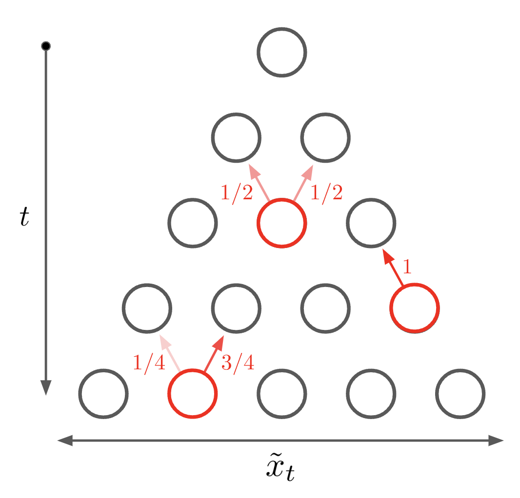
Figure 2. Left: example transition probabilities at various points in a reversed random walk. Center: simulated reversed random walks starting at $t = 100, x_t = 10$. The red curve shows the mean position. Right: simulated reversed random walks starting at $t = 1000, x_t = 40$. The red curve shows the mean position.

Jumps of many timesteps

In all our analysis so far, we’ve only tried to move forwards or backwards in time one step at a time. However, if we’re not interested in the intermediate trajectory, it’s easy to jump forwards multiple steps at a time, and it turns out we can do this backwards, too. Consider two times \(t, t'\) with \(t' > t\). Noting that the section of the random walk from \(t\) to \(t'\) is itself a random walk of length \(t' - t\), we find that

\[\begin{equation} \label{eqn:p_forwards_jump} p\left(x_{t'} | x_t\right) = 2^{-(t' - t)} \left( \begin{array}{c} t' - t \\ x_{t'} - x_t \end{array} \right). \end{equation}\]

With the same Bayesian approach as before, we can derive transition probabilities for a backwards jump. This yields that

\[\begin{equation} \label{eqn:p_backwards_jump} p\left(x_{t} | x_{t'}\right) = \frac{ \left( \begin{array}{c} x_{t'} \\ x_{t} \end{array} \right) \left( \begin{array}{c} t' - x_{t'} \\ t - x_{t} \end{array} \right) }{ \left( \begin{array}{c} t' \\ t \end{array} \right) }, \end{equation}\]

which reduces to Equation \(\ref{eqn:backward_step}\) when \(t' - t = 1\).

The continuum limit

While the discrete random walk is the easiest to grasp, in practice one often takes a continuum limit in which the walker’s motion is continuous in both time and space. This can be seen as the limit of a discrete-time random walk like the one studied above where, instead of taking \(\mathcal{O}(1)\) jumps with timesteps of size \(1\), our walker takes \(\mathcal{O}(dt^{1/2})\) jumps with timesteps of size \(dt\)³.

To get to the continuum, we’ll first switch from a discrete random walk to one in which the steps are sampled from a Gaussian distribution. This will make our walk continuous in space, which will simplify the subsequent process of making it continuous in time. We shall redefine our random walk as

\[x_0 = 0,\] \[\begin{equation} \label{eqn:forward_step_gaussian} x_{t+dt} \sim \mathcal{N}(x_t, dt), \end{equation}\]

where \(dt\) is a small constant step size and \(\mathcal{N}(\mu,\sigma^2)\) is a Gaussian random variable with mean \(\mu\) and variance \(\sigma^2\). Time-reversing this process with our same Bayesian trick, we find that

\[x_{t} \sim \mathcal{N}\left( \frac{ x_{t+dt} }{ 1 + \frac{dt}{t} }, \frac{ dt }{ 1 + \frac{dt}{t} } \right) \approx \mathcal{N}\left( \left(1 - \frac{dt}{t}\right) x_{t+dt} , dt \right),\]

where in the last step we’ve simplified assuming that \(dt \ll t\). Abusing notation a bit, we can write that

\[x_{t} \approx \left(1 - \frac{dt}{t}\right) x_{t+dt} + \mathcal{N}\left(0,dt\right).\]

We can now simply take \(dt \rightarrow 0\) and arrive at a differential equation for the continuum limit, finding that

\[\begin{equation} \label{eqn:sde} \frac{d x(t)}{-dt} = - \frac{x(t)}{t} + \eta(t), \end{equation}\]

where \(\eta(t)\) is the classic white noise process defined by having mean zero and covariance \(\mathbb{E}[\eta(t)\eta(t')] = \delta(t - t')\). This equation has a simple interpretation: this is an ordinary random walk with a pull towards the origin with strength \(t^{-1}\). The strength of this pull diverges as \(t \rightarrow 0\), sucking the walker in to \(x = 0\).

Neglecting the mean-zero driving noise and looking at only the drift term, we see that the mean of our distribution \(\mu(t) \equiv \mathbb{E}[x(t)]\) obeys

\[\frac{d \mu(t)}{-dt} = - \frac{\mu(t)}{t} \ \ \ \Rightarrow \ \ \ \mu(t) = C t\]

for some constant \(C\). This tells us that we expect that the mean of the distribution to approach zero linearly. Looking at the red curves in Figure 2, we see this is exactly what happens.

Chasing a moving target

Unlike the forward process, this reversed process isn’t stationary (i.e. time-translation invariant): as it runs, it approaches \(t = 0\), and its behavior changes. Stationary processes are nice, though; is there simple a way we could modify it to make it \(t\)-independent? One idea is to make it so the particle is chasing a moving target in a carrot-on-a-stick fashion: we fix some time \(T\) and “move” \(t=0\) so the random walk feels it is always a time \(T\) away from convergence. The end of this process will always appear to be a fixed time away, much like the advent of quantum computing or the release of Half Life-3. Mathematically, this corresponds to replacing \(t \rightarrow T\) in Equation \(\ref{eqn:sde}\), yielding

\[\frac{d x(t)}{-dt} = - \frac{x(t)}{T} + \eta(t).\]

This process is stationary and has an even simpler interpretation. In fact, neglecting the flipped direction of time, it’s exactly the classic Orenstein-Uhlenbeck process, which describes a random walker in a quadratic potential. Interestingly, the stationary distribution of this process is a centered Gaussian with mean \(\frac{T}{2}\), while from the forward walk we might expect it to have mean \(T\). I was surprised by this; I made some sense of it by noting that, if we started with the stationary distribution of \(x_T\) and applied many backwards steps, it’d contract to a narrower distribution, but it still feels weird to me.

Conclusions

So, what are the prospects for our Tenet-inspired video game? We’ve figured out how to model a simple random walk from the point of view of an observer moving backwards in time. It’s easy to imagine doing a similar thing for a walker with more complicated rules, like wandering around a map or interacting with objects. It’s also not too far-fetched to imagine rules that depend on the player, like a bias for moving towards the player or attacking with some probability, though we then run into the difficulty that the player’s future actions are unknown (a problem that’s a cousin of our earlier paradoxes regarding free will). This blocks our Bayesian calculation and needs a clever trick or two to give a good game mechanic. If you’re game-design-minded and interested in thinking through this further, feel free to reach out!

Note on the genesis of this post

This idea was largely inspired by a post-Tenet conversation with Vishal Talasani. This writeup was made by starting with a blank file and randomly hitting a time-reversed delete key until it was done.

Footnotes