Multiplicative neural networks
Introduction
In the past decade, neural networks have proven to be stunningly effective tools for a slew of machine learning tasks as diverse as classifying images, generating 3D graphics, and playing games. These incredible successes all stem from neural networks’ remarkable ability to perform a central task in machine intelligence: given complex data, find underlying patterns.
Boiled down to their core, neural networks are just a series of hierarchical nonlinear transformations. Each layer of the neural network is one layer in this hierarchy, transforming a feature vector and passing it to the next layer up, until it reaches the output. Each layer usually involves a step that mixes the elements of the feature vector according to a set of weights followed by a nonlinear function applied to each element of the vector. All types of neural networks use a series of these layers to do the basic information processing.
Within that hierarchical nonlinear structure, however, there are many variations. There are a vast array of different ways layers can be connected and parameterized, giving different architectures like convolutional nets, recurrent nets, and resnets specialized to certain types of task. However, there are also lower-level things that can be changed. One example is the nonlinear function, usually denoted \(\sigma\). The field’s explored many options for \(\sigma\) over the years, and the most popular choice has changed over time. The \(\tanh\) function (and similar sigmoid) were once the leading choice, but the \(\text{ReLU}\) (defined by \(\sigma(x) = \max(x, 0)\)) is now more popular. Choosing a different nonlinearity can improve performance slightly, but to me it is more striking that the choice of nonlinearity matters so little. On the face of it, the \(\text{ReLU}\) and \(\tanh\) functions are basically as different as they could be within reason. \(\tanh\) is smooth, saturating, nonlinear on every finite set, and is symmetric about the origin. \(\text{ReLU}\) has a kink, is unbounded, piecewise-linear, and never takes negative values, not to mention that it outputs zero on half of its domain. The fact that both of these functions could work reasonably well speaks to the fact that even though the hierarchical nonlinear structure is core to the effectiveness of neural nets, the exact choice of nonlinearity is, surprisingly, not crucial.
In fact, even the typical layer structure of matrix multiplication + elementwise nonlinearity isn’t crucial to performance. It has been shown that tensor networks, a completely different type of hierarchical nonlinear model commonly used in physics, can also learn machine learning tasks. This paper develops the idea and gets 1% test error on MNIST, which is pretty good for a totally new approach. Interestingly, neural networks have recently been used instead of tensor networks in computational physics problems and achieved good performance there. This raises a natural question: how do we know that the matrix multiplication + elementwise nonlinearity structure is really the best one? To my knowledge, there’s no known fundamental, theoretical reason why it would be better than other options.
Multiplicative nets
Here’s an idea for a different type of nonlinear hierarchical model. What if we took a neural network and replaced the matrix multiplication step \(\sum_j w_{ij} x_j\) with a product step \(\prod_j x_j ^ {w_{ij}}\), with the weights as exponents in a product instead of coefficients in a sum? This would still mix together the elements of the feature vector \(x\), just like a matrix operation, but in a different, nonlinear way. Given the way deep learning systems can sometimes be surprisingly invariant to details of implementation, maybe this new, different sort of model could still work well.
Architectures using this idea are called multiplicative neural networks. The idea was first proposed in 1989 by neuroscientists seeing multiplication as more biologically plausible and potentially more powerful than addition. They were tested experimentally on some very small problems in the next decade and once analyzed from a complexity standpoint in the decade after. The architectures these papers describe are a little more general - they consider combining additive and multiplicative neurons in the same net and using hybrid terms with more weights of the form \(v_1 \prod_j x_j ^ {w_{ij1}} + v_2 \prod_j x_j ^ {w_{ij2}} + ... + v_n \prod_j x_j ^ {w_{ijn}}\) - but their key innovation is the multiplicative form. However, despite this research, multiplicative nets never broke through to practical use; we still use additive neural networks with normal matrix operations.
This is pretty understandable - at a first glance, multiplicative nets seem like they’d have some problems. One immediate question is what to do when \(x_i < 0\) and \(w_{ij}\) isn’t an integer, in which case \(x_i ^ {w_{ij}}\) isn’t uniquely defined, but to avoid that problem let’s just set things up so that all the \(x_i\) are positive, which I’ll show we can do with the right choice of data and nonlinearity. Even dealing with this, though, these nets have some pretty prolific potential practical problems. First, there’s been a lot of research and hardware development into making matrix operations faster, and this wouldn’t use them. Second, replacing simple matrix operations with something more complex could lead to weird gradients and failed optimization. Third, as a friend noted, even from a pure computational complexity standpoint, calculating \(x^y\) is more expensive than calculating \(x*y\), so this would be slow. Finally, the advantages of switching to this architecture are far from clear, so there’s no incentive to overcome these problems.
The purpose of this post is to explore something interesting that isn’t discussed in the above papers: the multiplicative nets you get by replacing \(\sum_j w_{ij} x_j\) with \(\prod_j x_j ^ {w_{ij}}\) are basically identical to normal, additive neural nets with a different choice of nonlinearity. The basic reason is that, as the 1989 paper did note, \(\prod_j x_j ^ {w_{ij}} = \exp \big( \sum_j w_{ij} \ln(x_j) \big)\), so a multiplicative layer is the same as an additive layer where you take the logarithm before and an exponential after. The main trick we’ll use is the fact that you can then absorb the \(\ln\) and \(\exp\) into the nonlinearity to get a new nonlinearity \(\sigma'(x) = \exp\sigma(\ln(x)))\), or, with compositional notation, \(\sigma' = \exp \circ \sigma \circ \ln\).
My argument could easily be laid out with standard symbolic math. However, that’s not how I think about it, and I don’t think it’s the clearest way to explain it. Notation matters; different ways of writing the same thing inspire different kinds of manipulations, and cleaner notations are better to learn with. Instead of algebra, I’ll use diagrams.
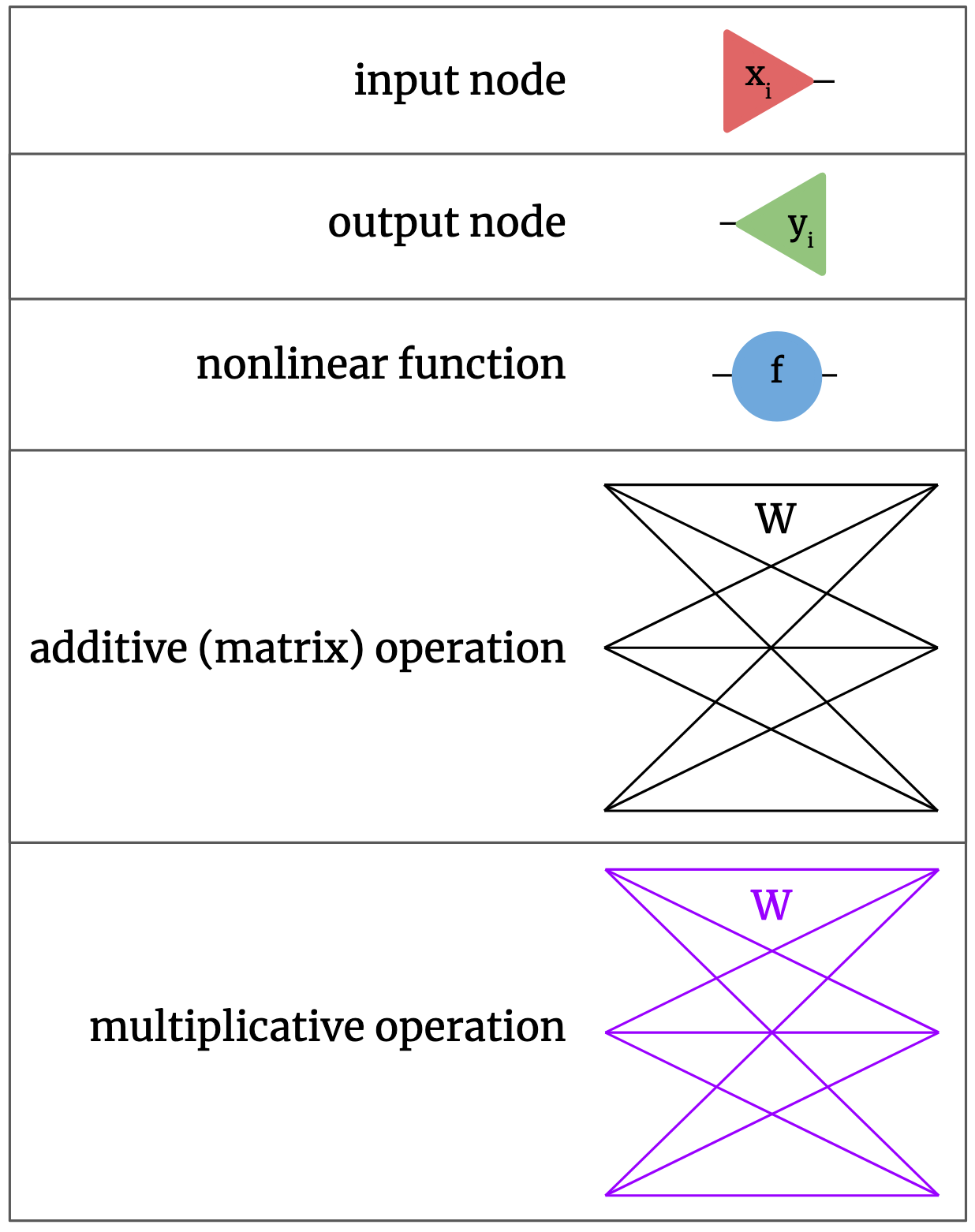
Basic neural nets are built of a few basic pieces. There are input nodes, where input data vectors go into the net. There are output nodes, where the net’s output comes out. There are elementwise nonlinear functions, mapping real numbers to real numbers. There are additive or matrix operations, each with its own 2D array of parameters \(W\), which in normal neural nets come between applications of nonlinear functions. Lastly, we’ll include multiplicative operations, which also each have their own 2D array array of parameters \(W\) as discussed above. We’ll use color to differentiate between additive and multiplicative operations; additive will be black, multiplicative will be purple. Note that changing an operation from additive to multiplicative or vice versa doesn’t change its parameter matrix; the same numerical weights are just interpreted differently in a different operation. We could also add pieces like biases or specialized layers like softmax or maxpooling, but we’ll leave those out for now for simplicity. We could cast these pieces into diagrammatic form as follows:
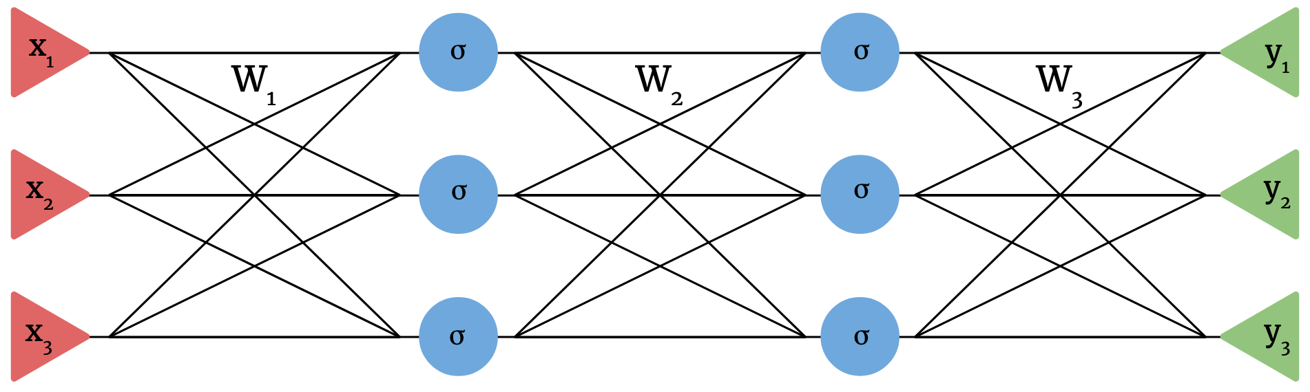
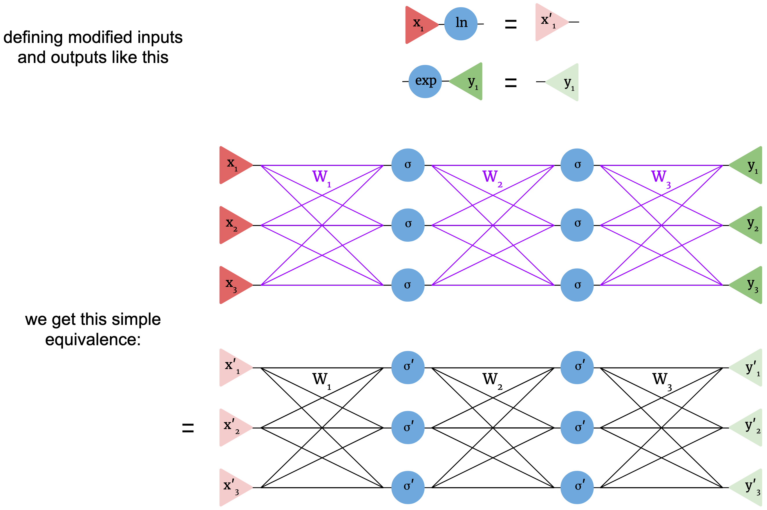
We can now build neural nets out of these components. For example, the following is a standard additive neural net with 3-dimensional input, 3-dimensional output, two hidden layers with width 3, and a nonlinearity \(\sigma\).
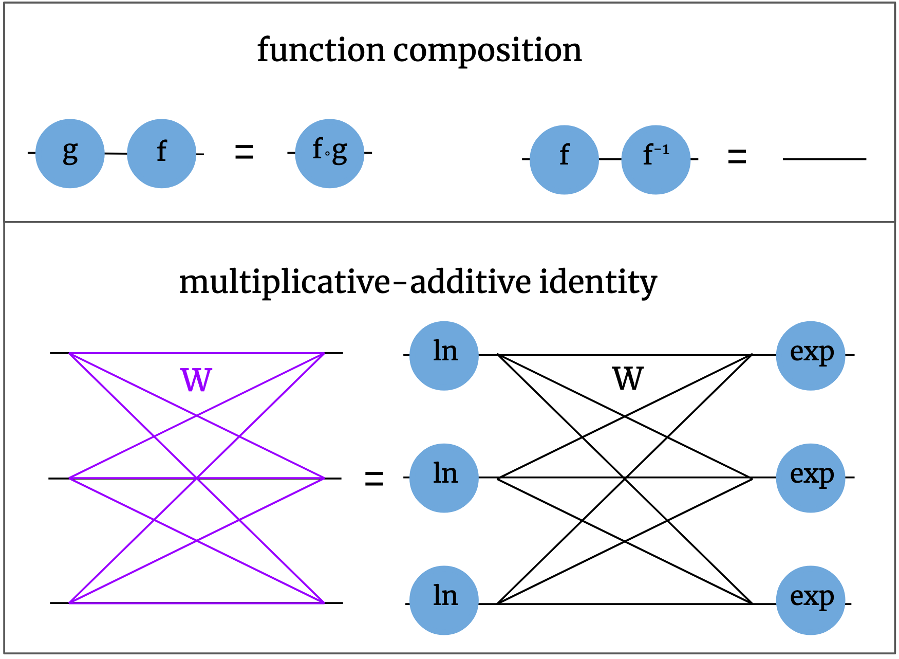
There are a few different ways we can manipulate these diagrams while still keeping the model the same. The first way is function composition. If there are two nonlinear functions in a row, we can just replace them with one new function. This is just saying that the double function application \(f(g(x))\) is equivalent to the single function application \(h(x)\), defining \(h = f \circ g\). One special, familiar case is when the two functions are each other’s inverses, and the new function is simply the identity; for example, \(\ln(\exp(x)) = x\). Instead of writing the identity function explicitly, we can just write a line. Note that in the notation \(f \circ g\), functions are applied right to left, but in our diagramas, everything flows from left to right, so the ordering of the composed functions might seem backwards at first. There’s also the multiplicative-additive net identity we talked about earlier: \(\prod_j x_j ^ {w_{ij}} = \exp \big( \sum_j w_{ij} \ln(x_j) \big)\). A multiplicative layer is the same as an additive layer with logarithms before and exponentials afterwards. We can write these rules like this:
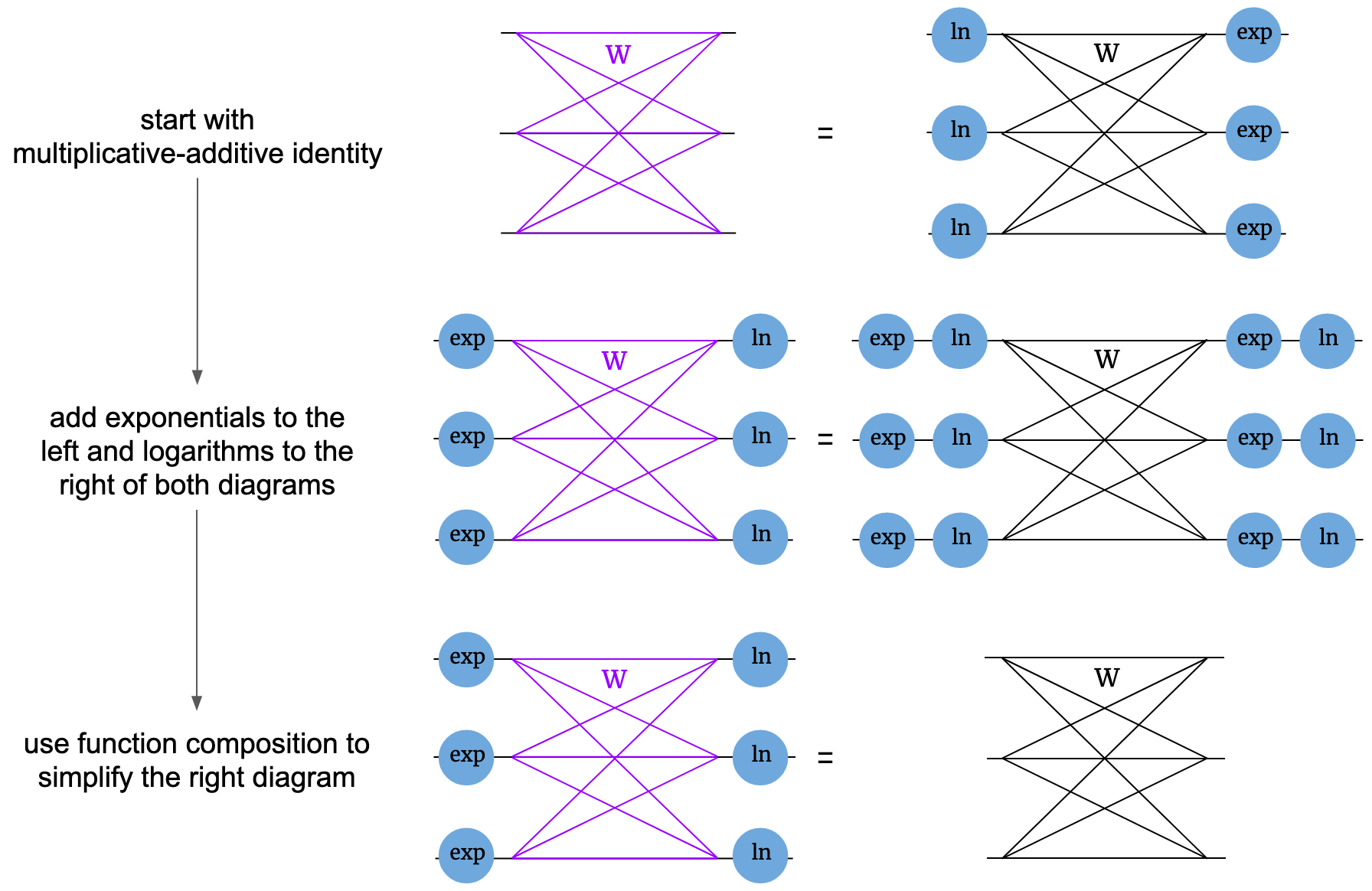
These rules lay out ways we can manipulate diagrams. As a test of this notation, with just these simple rules we can derive a companion rule to the multiplicative-additive identity. Just as you can take a function of both sides of an algebraic equation, we’re allowed to modify a diagrammatic equation by attaching pieces to dangling ends of both diagrams in the same way. In this case, we’ll attach exponentials on all dangling ends on the left and logarithms on the right of both diagrams. This gives us a new diagrammatic equation. We can then use function composition to simplify the adjacent logarithms and exponentials to get a new, simple identity. This one tells us that \(\ln \big( \prod_j \exp(x_j)^{w_{ij}} \big) = \sum_j w_{ij} x_j\), which you can algebraically check is true.
Now, let’s put together a multiplicative net and see what we can derive. Our starting point will be the same simple 3-3-3-3 net as before, but with multiplicative layers; it will be clear that our operations will generalize to different sizes. First, we use the multiplicative-additive identity to get an additive net. However, instead of just having one nonlinear function acting on each element of the feature vector, there are now three in succession. Using function composition, we can just group these into a new nonlinearity we define as \(\sigma' = \ln \circ \sigma \circ \exp\). We now arrive at an additive net exactly equivalent to the multiplicative net. The only major oddity of the new additive net is elementwise logarithms at the start and exponentials at the end.
![]()
These logarithms and exponentials at the start and end aren’t surprising. We’re requiring that multiplicative nets need positive input and give positive output, so since logarithms of negative numbers aren’t real, these logarithms enforce the positivity of the input. The exponentials similarly enforce the positivity of the output. Also, as long as \(\sigma\) maps positive numbers to positive numbers, the net only operates on positive numbers intermediately, and we don’t have the undefined power problem. We can make our diagram even simpler by absorbing the logarithms and exponentials into the inputs as follows:
It turns out that a multiplicative net is basically the same as an additive net with the same weights! Our choice of notation emphasizes the similarity of form. However, is this really a meaningful, useful correspondence? The main question is this: what’s the nonlinearity \(\sigma'\) like? It’s possible that \(\sigma' = \ln \circ \sigma \circ \exp\) is some bizarre function that’d be totally nonfunctional in an additive net, which would bode badly for our multiplicative net. To answer this, a few examples are plotted below. The blue curves show different choices of nonlinearity for multiplicative nets, defined only for positive inputs, and the orange curves show the corresponding additive nonlinearities.
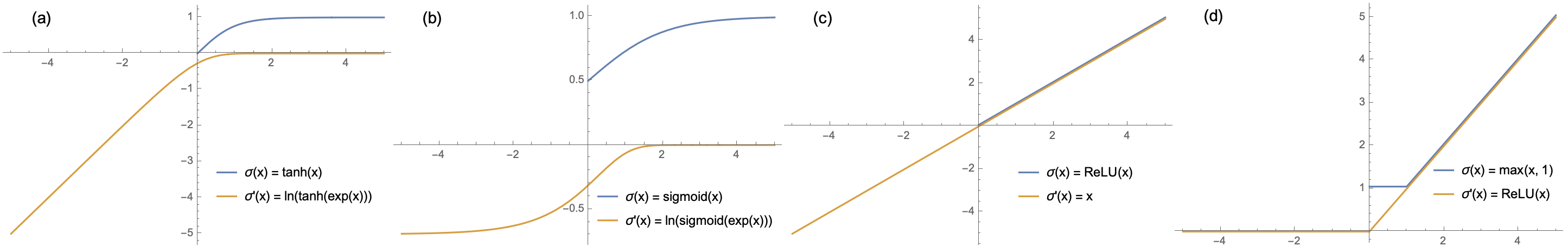
As shown in (a), when \(\sigma\) is the \(\tanh\) function, \(\sigma'\) looks a lot like a smoothed \(\text{ReLU}\), also called a softplus! It’s flipped across the x- and y-axes, but that doesn’t change the usefulness of a nonlinearity in an additive neural net. This would definitely work as an activation function. Surprisingly, (b) shows that when \(\sigma\) is a sigmoid, \(\sigma'\) is also roughly a sigmoid (but again flipped across both axes), which also works as a nonlinearity. Shown in (c) is the case when the multiplicative net uses a \(\text{ReLU}\) nonlinearity. This is a distinctly horrendous choice for only positive inputs, since it’s the same as the identity on positive input, which is reflected in the fact that \(\sigma'(x) = x\). A multiplicative neural net with \(\text{ReLU}\) nonlinearities is basically linear; adding extra layers doesn’t give it any power since, for additive networks, a multilayer linear net is reducible to a linear model. With a slight modification, however, we get a very useful nonlinearity. As shown in (d), if the nonlinear net uses a modified \(\text{ReLU}\) - specifically, \(\sigma(x) = \max(x, 1)\) - the corresponding linear net has exactly \(\text{ReLU}\) activations.
It might not be clear what, exactly, this means for multiplicative nets. Let’s suppose that we’re using a multiplicative neural net to do a task - say, classifying images - and we operate it by exponentiating the pixel values at input and taking the log of the output. We have shown that, for a reasonable nonlinearity, the function the multiplicative net computes as a function of weights and data - say, \(f(X ; W)\) - is exactly the same as for a reasonable additive net. That means that the loss surface is the same. That means that the gradients are the same, and that means that the trainability is the same, and all this means that the theoretical usefulness of multiplicative neural nets, including their representational power and optimization behavior, are the same as the standard additive neural nets that have been the focus of such intense study. Multiplicative nets are just as effective, there’s a correspondence to additive nets, and we have the conversion algorithm.
This fact is intriguing, but what does it mean in a broader sense? This doesn’t make multiplicative nets practically useful; it’s still faster to perform a matrix multiplication than a multiplicative step, and since they amount to the same thing there’s no reason to prefer the latter. To me, the reason this fact bears consideration is the hint it might be towards what truly gives deep learning its unreasonable effectiveness. Multiplicative and additive nets have starkly different functional forms, and at a first glance I’d guess they have wholly different behavior as models. The fact that they actually have equivalent power and utility seems like a hint that the fundamental magic of deep learning doesn’t lie in the details of implementation, like the choice of activation function or even the choice of matrix multiplication for mixing; the latter’s just preferred for convenience. It seems likely that the key to deep learning’s success is something more deep and general about hierarchical nonlinear structures, and wildly disparate hierarchical models, from standard neural nets to multiplicative nets to tensor networks, all succeed because in some deep way they all fit this broad category. Perhaps efforts to understand deep learning will eventually uncover a mathematical understanding of something like this.
Extras
-
“Wait,” you might say, “there’s no clean correspondence to an additive net if the multiplicative net has a more complicated form, like involving a sum of product terms. This analysis only works in one case when it happens to be trivial!” It’s true that the exact correspondence is easy to break by adding a bell or a whistle to the multiplicative net. The question, however, is whether these modifications add anything fundamentally different, or whether they’d be incremental changes at most. I can only conjecture for now - maybe I’ll do experiments if this becomes a paper - but I’d guess it’s likely that there are many ways to superficially change the form of multiplicative nets without fundamentally changing their behavior because the same is true of additive nets. For example, you can add extra parameters to neural nets by parameterizing the activation functions themselves; this paper not only tried that, but ran an evolutionary algorithm to build complicated activation functions, and their error rates were only a few percent lower than with simple \(\text{ReLU}\)s. Many such engineering intricacies lead to no big change in performance. For that reason, I think it’s a decent hypothesis that multiplicative nets behave similarly to additive nets even when there’s no exact correspondence.
- In the diagrams I drew, the nets have only weights, not biases. Since \(\exp \big( \sum_j w_{ij} \ln( x_j ) + b_j \big) = e^{b_j} \prod_j x_j ^ {w_{ij}}\), we can add them by multiplying the product by \(e^{b_j}\), where \(b_j\) is a new bias parameter.
- The choice of base \(e\) (i.e. \(\exp\) and \(\ln\)) in this article was arbitrary, and any other base would’ve worked.
- Many types of specialized neural net layer can also be translated into multiplicative nets. For example, a softmax is similar, but it doesn’t even require taking the exponentals. \(\exp\) and \(\ln\) are monotonic, so they commute through max operations, so maxpool layers are the same for multiplicate nets.
- Are there other choices for the mixing operation besides the matrices of additive nets and the multiplication operation shown here? One way to generalize the concept to include both is to make the mixing transform \(f \big( \sum_j w_{ij} f^{-1}(x_j) \big)\), with \(f\) an invertible function mapping reals to reals. In the case of \(f = \text{identity}\), this gives additive nets. In the case of \(f = \exp\), this gives multiplicative nets. In a case like \(f(x) = x^3\), though, it would give something new, but still equivalent to an additive net by the same sort of proof.
- The most recent paper I’ve found on these nets, which was mentioned above, argues that multiplicative neurons perform operations that need large numbers of summing units, stating that “networks of summing units do not seem to be an adequate substitute for genuine multiplicative units.” This post basically disproves that!