The principle of least power dissipation
I’m currently in a class called Physics of Computation on new types of computing paradigms that don’t solve problems in discrete, sequential, logical steps like modern computers. Instead, the whole computing system goes through a complex analog evolution, with every variable free to change simultaneously, and eventually settles into a stable final state representing the answer. Naturally, one of the core challenges is in designing a system that predictably settles into a steady state with some desired properties.
Our professor’s pointed out that many such computing systems can be seen to accomplish this by using a little-known concept called the ‘principle of least energy dissipation.’ When a battery or current source is hooked up to a DC circuit, a sudden flow of current flares through the different branches of the circuit, sometimes much more or less at first than is sustainable. Eventually, though, these initial errors fade away, and the circuit ends up in a steady state, with currents and voltages everywhere that don’t change in time. The principle of least energy claims that of all the possible steady states satisfying the voltage and current constraints, the real steady state dissipates the least amount of power.
I’ve solved tons of DC circuits, and I’d never heard of this. To my shock, though, it worked for a few simple circuits we discussed in class. However, these simple examples neither showed it always works or explained why it does. To try to understand, I read Feynman’s lecture on minimization principles; it turns out that at the end he mentions this law but doesn’t really explain it, so I decided to fill in the gap.
It’s actually easier to see that it’s true if you start with a general, continuous 3D system; everything’s captured in one differential equation instead of having to deal with discrete voltages and resistors. Suppose we have a volume \(V\) filled with a resistive medium with resistivity \(\rho(\mathbf{r})\). It could have different resistances at different points; that’ll be important later. Now, suppose there’s an electric potential (a voltage) \(\phi(\mathbf{r})\) throughout the medium. We also need some way to add a constraint to the system (like plugging a source into a circuit), so we’ll suppose that the potential at the surface is completely fixed; perhaps it’s higher at one end and lower at the other to cause a current flow. In real circuits, currents cause magnetic fields that can affect charges a little, but we’ll ignore magnetism for this problem.
The currents and voltages throughout a resistive circuit are determined entirely by the sources and the circuit structure, so we expect that \(\phi\) and the current should be determined entrely by boundary conditions and \(\rho\). How do we find them? Well, the typical way is to say that the potential corresponds to an electric field \(\mathbf{E}(\mathbf{r}) = - \mathbf{\nabla}\phi\) which then creates a current \(\mathbf{J} = \rho^{-1} \mathbf{E}\) according to the continuous version of Ohm’s Law. In the steady state, charge isn’t building up anywhere, which implies that \(\mathbf{\nabla} \cdot \mathbf{J} = -\mathbf{\nabla} \cdot (\rho^{-1} \mathbf{\nabla} \phi) = 0\). Solving this to match the boundary conditions on \(\phi\) gives the potential, which gives the current. Note that this would reduce to \(\nabla^2 \phi = 0\), which you might recognize as the equation voltage satisfies when there’s zero charge density, if \(\rho\) were a constant; the reason it doesn’t is that, even in steady-state DC circuits, there’s actually built-up charge on the interfaces between components of different resistivities.
Let’s see if we can derive that differential equation not by assuming that \(\mathbf{\nabla} \cdot \mathbf{J} = 0\) but just by assuming that the power dissipation is as small as possible. The total power dissipation is given by \(P = \int_V (\mathbf{J} \cdot \mathbf{E}) \mathop{}\!\mathrm{ \mathbf{dr} } = \int_V \rho^{-1} (\mathbf{\nabla}\phi)^2 \mathop{}\!\mathrm{ \mathbf{dr} }\). Feynman’s lecture neatly explains how to find minimal solutions, so I’ll just tear through the steps quickly. Since we’re looking for a minimum, we want to find a choice of \(\phi\) that makes \(P\) invariant to perturbations to first-order. If we add a small perturbation \(\delta\phi\) to \(\phi\), so the new potential field is now \(\phi + \delta\phi\), the power dissipation becomes \(P + \delta P\), where \(P\) is the same as before and \(\delta P = 2 \int_V \rho^{-1} \mathbf{\nabla}\phi \cdot \mathbf{\nabla}(\delta\phi) \mathop{}\!\mathrm{ \mathbf{dr} }\). The usual integration by parts trick gives \(\delta P = -2 \int_V \mathbf{\nabla} \cdot \big[ \rho^{-1} \mathbf{\nabla}\phi \big] \delta\phi \mathop{}\!\mathrm{ \mathbf{dr} }\), and since \(\delta\phi\) was arbitrary, this implies that \(-\mathbf{\nabla} \cdot (\rho^{-1} \mathbf{\nabla} \phi) = 0\)! That’s it - minimizing power dissipated is equivalent to the same steady-state differential equation you get from working through the electrodynamics the normal way. Any \(\phi\) that minimizes power dissipation is a real physical solution, and any physical solution minimizes power dissipation.
The math is all well and good, but how can we really understand it? What’s the physical reason why power should be minimized? Well, the differential equation we derived from power minimization is just the fact that the current \(\mathbf{J}\) has zero divergence. That actually makes sense in terms of minimizing power dissipation! Imagine a point in the medium with nonzero current divergence, so it’s a sink (or a source) of current. In the vicinity of that point, on top of whatever divergence-free flow there is, there’s an extra part of the current that flows into or out of the point. In a rough sense, it turns out that you can decrease the dissipated power by just dropping that extra part of the current.
That’s the case of a problem where the voltage is prescribed. Circuits can have both voltage and current sources, though; what about a case where the current on the boundary is given? Well, first, it’s important to note that only the current normal to the boundary can be prescribed; to illustrate why, if you could prescribe arbitrary currents on the boundary, you could have the current flow in a circle around the boundary, which we know is already unphysical. We’ll also have to assume that \(\mathbf{\nabla} \cdot \mathbf{J} = 0\) - if we just let charge accumulate in the medium, the minimum power dissipation solution will just be to have zero current everywhere and have charge build up forever on the surface. However, if we again minimize power dissipated using vector calculus tricks, we get a new, interesting condition: \(\mathbf{\nabla} \times (\rho\mathbf{J}) = 0\); the curl of \(\rho \mathbf{J}\) is zero. Since curl-free vector fields are gradients of potentials, this gives us the condition that \(\mathbf{J} = -\rho^{-1}\mathbf{\nabla}\phi\) for some potential \(\phi\), and since we assumed the current has zero divergence, this gives us \(-\mathbf{\nabla} \cdot (\rho^{-1} \mathbf{\nabla} \phi) = 0\)! Again, the new condition that minimizing power dissipation bought us actually makes physical sense; if the curl of \(\rho \mathbf{J} = \mathbf{E}\) weren’t zero, there would be current flowing uselessly around in loops and dissipating extra power.
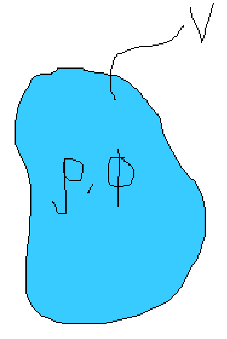
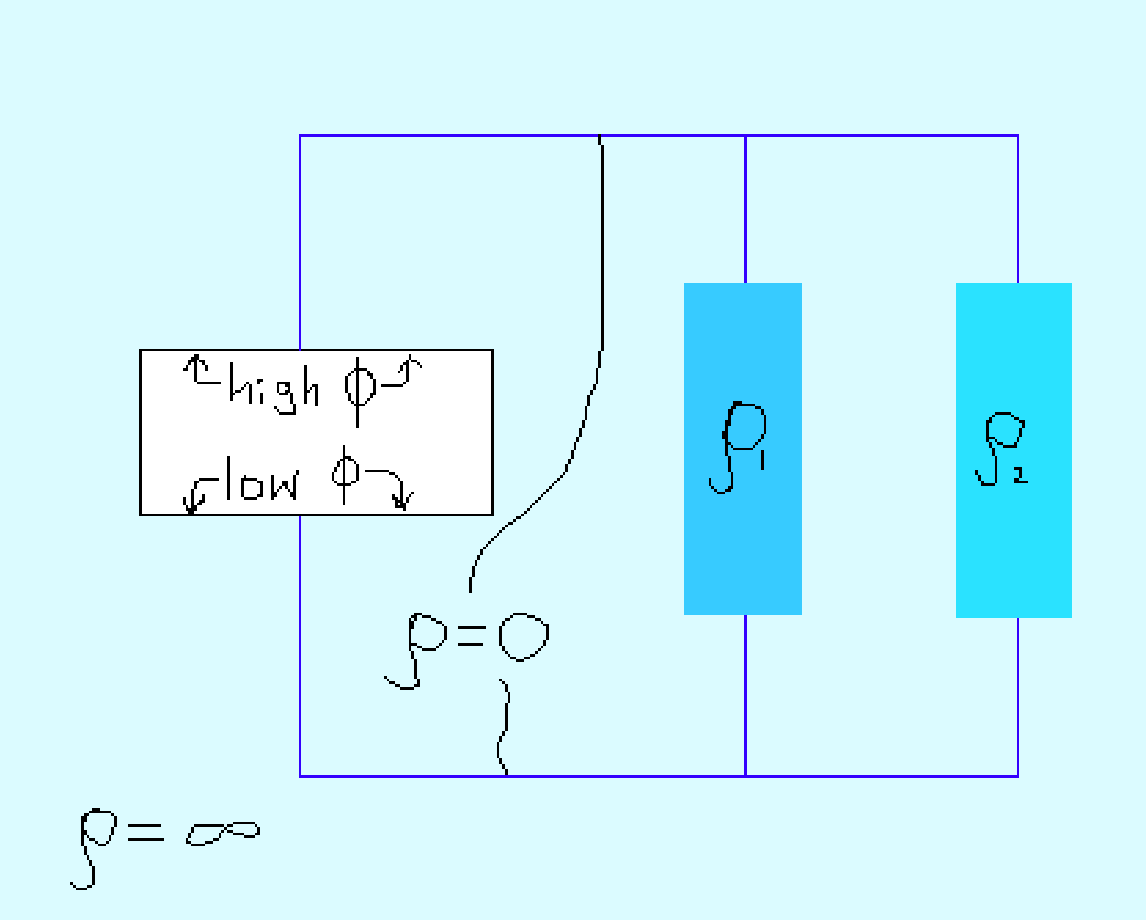
Alright, now we’ve decently explained why power dissipation is minimized in scenarios when current’s flowing through a continuous resistive medium. We were originally interested in circuits, though; how does this relate? We can actually cleverly fashion a resistive circuit by just changing \(\rho(\mathbf{r})\)! For most of the volume, we’ll let \(\rho \rightarrow \infty\), which turns it into a very good insulator, like the air between the wires in a circuit. Then we’ll let \(\rho \rightarrow 0\) in some long, thin regions that will become wires. Along the wires we’ll make some regions have intermediate values of \(\rho\), which makes them resistors. Lastly, if we want, we can choose our boundary so all of space except where a source will go is enclosed in it, then specify the voltage or current along the boundary. This gives a circuit of sources, wires and resistors that might look as follows:
Now we have a circuit. How does minimal power dissipation explain its current and voltage distribution? From the point of view of choosing voltages at each node of the circuit, any voltage distribution besides the true one will lead to charges accumulating somewhere, which requires some extra current and dissipates extra power. From the point of view of choosing how currents branch at every node, any split besides the true one will correspond to extra current running around in a loop, which wastes power, and also an electric field with a nonzero curl, which doesn’t correspond to a potential.
We’ve shown that the principle of least power dissipation gives the right answers for steady-state circuit problems. If this is really a general law of nature, though, it’d probably show up outside of just this one narrow context. It turns out that it can also be applied to fluid circuits, which are sometimes studied as somewhat-similar sister systems to electric circuits. In the sort of fluid circuit I’m imagining, there are networks of pipes of different thicknesses instead of resistors with different resistances. Water flow rate \(Q\) replaces current, pressure \(P\) replaces voltage, the rate of power dissipation is \(PQ\) instead of \(VI\), and pipes have an effective resistance. An ideal pipe with laminar flow has \(\Delta P\) proportional to \(Q\) in an equation analogous to Ohm’s Law, and the quantity analogous to resistance depends on the pipe’s dimensions and the viscosity of the fluid. The fact that these equations map onto each other so perfectly means that fluid through a network of pipes minimizes power dissipation just as electrical circuits do. I’d be willing to bet that, just as we derived part of the differential equation for current flow, you could derive part of the Navier-Stokes equations just from minimizing power dissipation.