Insights into GPT-2's positional encodings
In this blogpost, I show that GPT-2’s positional encodings lie in a roughly orthogonal subspace to its token embeddings. I then show that the subsequent attention layer and MLP are sensitized to these subspaces in intuitive fashions.
I’m finally learning about transformers, and I intend to both learn the factual basics and also build up some intuition for how they work and how to think about them. In doing so, I found I got a bit stuck when reading about positional encoding, the original scheme used to provide transformers with token position information. In particular, I was confused as to how the positional encodings wouldn’t interfere with the token embeddings. Messing around with GPT-2, I found the answer’s basically that they’re learned to be orthogonal, and the consequences of this can be seen in downstream weight tensors, too! I’ll begin by framing the puzzle here, then show numerical evidence that these two types of embedding are approximately orthogonal, and finally show how this is reflected in some model weight tensors.1
Introduction: why don’t positional encodings interfere with token embeddings?
The attention operation at the core of modern transformer models is blind to the order of the embedding sequence it takes as input. The operation cares only about the similarity (as computed via the attention mechanism) between two token embeddings in the sequence and is blind to their absolute and relative positions in the sequence (except for the causal mask, which we’ll ignore). This positional information is important, though, so it’s typically given to the model via positional encodings.
Under this scheme, after the input sequence is tokenized and mapped to initial token embeddings, a unique vector representing a token’s index in the sequence is added to each embedding. This provides token position information to the downstream model. Mathematically, if our input is a sequence of tokens ${x_0, x_1, x_2, \ldots }$, we first apply a token embedding map $E$ to get a sequence of vectors ${E(x_0), E(x_1), E(x_2), \ldots}$ and then add positional encoding vectors ${p_i}$ to each embedding vector to get ${E(x_0) + p_0, E(x_1) + p_1, E(x_2) + p_2, \ldots}$. The result is a sequence of embedding vectors such that each vector $e_i = E(x_i) + p_i$ is aware of both its input token $x_i$ and its index $i$. This sequence is then passed on to the rest of the transformer.
Thinking through the vector math here, the choice to simply add positional encodings to the token embeddings seems surprising. I’d naively expect these vectors to interfere with each other! We’d ideally like to be able to easily resolve both the token embedding and its position, but by adding the corresponding vectors, we get some superposition that sort of muddies them together.2 This is weird because you’d imagine the downstream circuitry will want to be able to resolve the two.
This wouldn’t be a problem if the operation were vector concatenation instead of addition. Equivalently, this wouldn’t be a problem if we were knew that the token embeddings and positional encodings lie in roughly orthogonal subspaces, so they won’t interfere. This seemed like a reasonable enough hypothesis that I looked at GPT-2’s encoding to check, and it turns out that this is basically what’s happened — the embeddings and encodings learn to lie in roughly orthogonal subspaces!
Claim: [positional encodings] $\perp$ [token embeddings]
Here I will present numerical evidence that the positional encodings and token embeddings lie in roughly orthogonal subspaces. I’ll first plot the singular values of both embedding matrices, which will show that the positional encodings concentrate in a pretty low-dim subspace, then show that this subspace is roughly orthogonal to the space of the token embeddings.
Let’s fix some notation. GPT-2 has an embedding dimension of $d_\text{model} = 768$, a vocabulary size of $d_\text{vocab} \approx 50 \times 10^3$, and a max context window of size $d_\text{context} = 1024$. We’ll denote the token embedding matrix by $\mathbf{E} \in \mathbb{R}^{d_\text{vocab} \times d_\text{model}}$ and the positional encoding matrix by $\mathbf{P} \in \mathbb{R}^{d_\text{context} \times d_\text{model}}$. Here are the singular values of these two matrices:
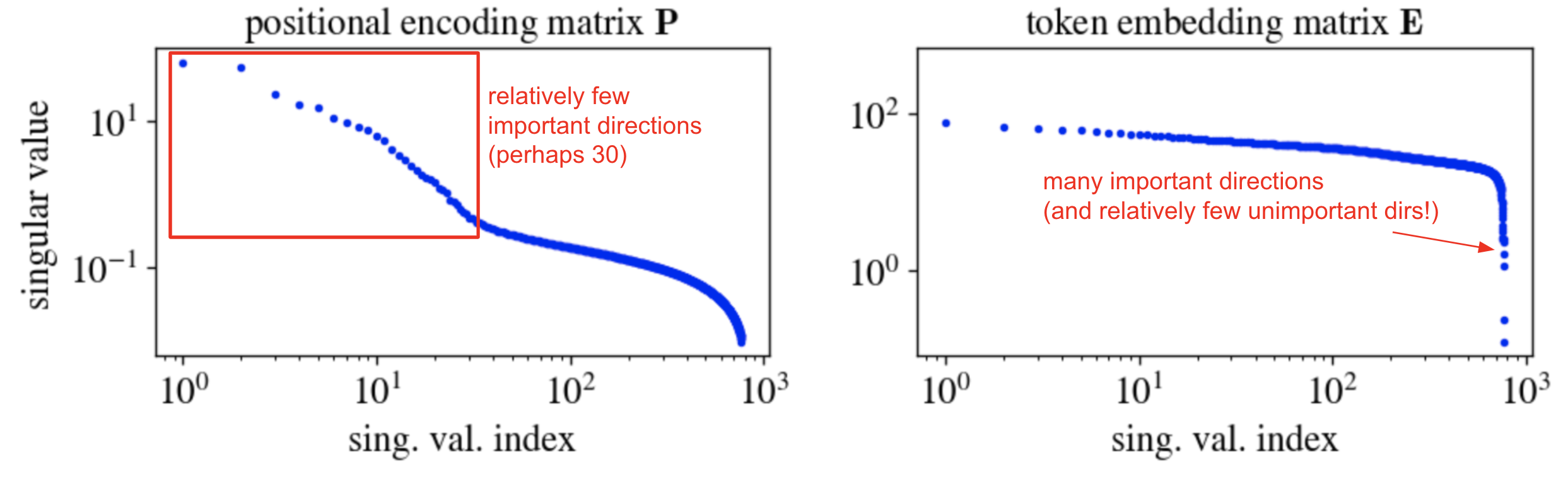
The most important observation here is that $\mathbf{P}$ has fairly low rank: it’s very well captured by its top, say, 30 singular directions. The embeddings, by contrast, have fairly high rank: the mass of $\mathbf{E}$ is spread over many singular directions.
We will now show that the top directions of the right singular subspace of $\mathbf{P}$ (which capture most of its mass) align well with the bottom directions of the right singular subspace of $\mathbf{E}$, which permits them to not interfere with each other. Let the right singular vectors of $\mathbf{E}$ be $v_j$ for $j = 1, \ldots, d_\text{model}$, and let \(\Pi^{(30)}_\mathbf{P}\) be the projector onto the top 30 right singular directions of $\mathbf{P}$. The plot below shows \(v_j^\top \Pi^{(30)}_\mathbf{P} v_j\). This quantity lies in $[0,1]$ for each index $j$ and tells us the degree to which each embedding singular direction is captured by the top singular directions of the positional encoding matrix.
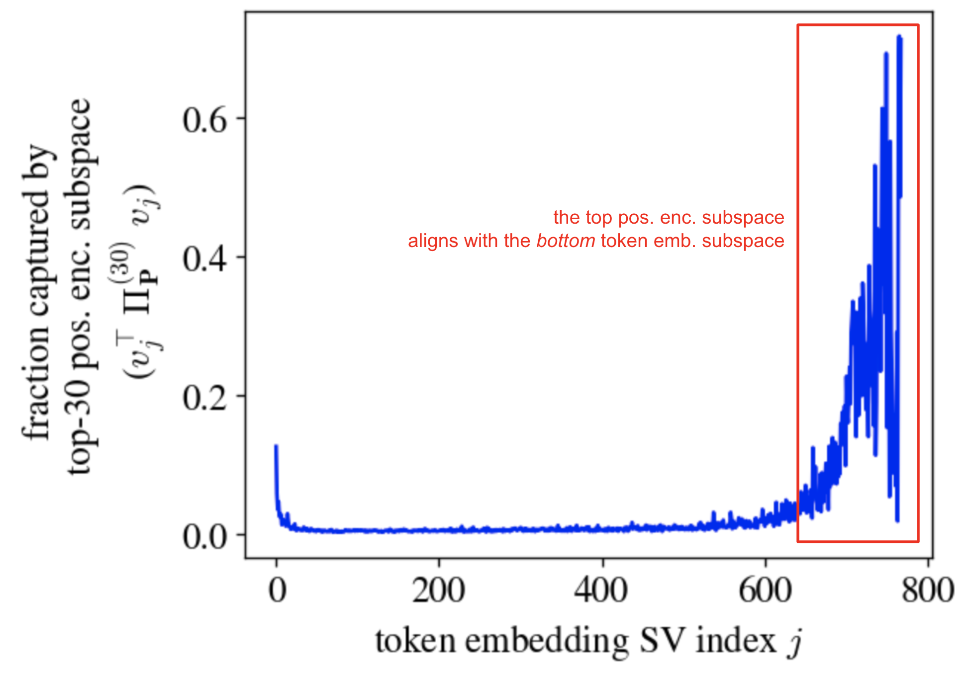
The large mass towards the right of the above plot shows that the top subspace of the positional encodings is well-aligned with the bottom subspace of the token embeddings. Phrased differently, the positional encodings and token embeddings lie in roughly orthogonal subspaces, and so they won’t interfere!
Curiously, the above plot also shows a small mass at the low indices. This is strange to me, and I don’t know what to make of it. Feel free to send me hypotheses!
Here’s another, more detailed viz of the same phenomenon. Here I simply plot the squared overlaps of the right singular vectors of $\mathbf{P}$ and $\mathbf{E}$:
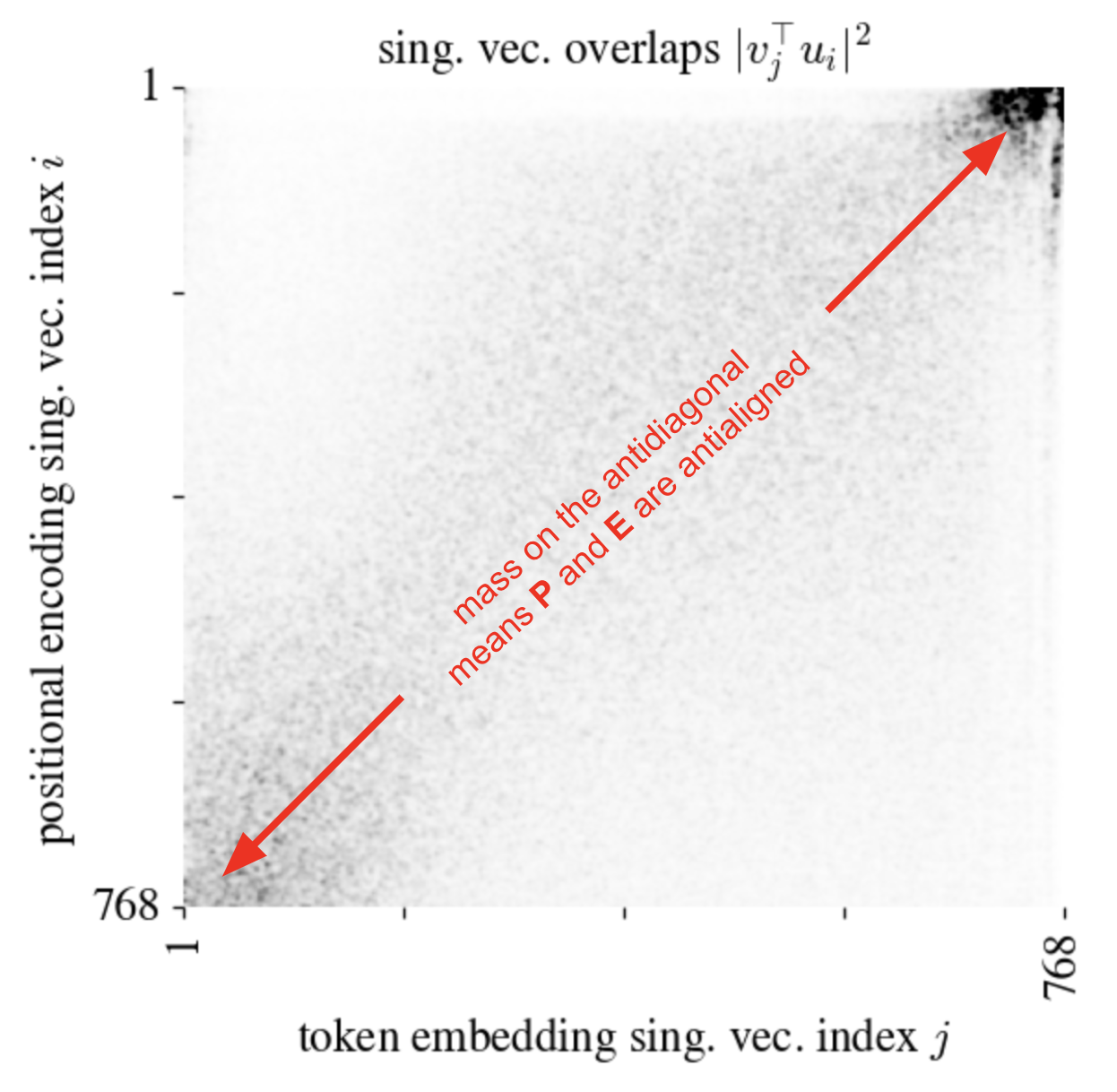
I’ve applied a small Gaussian blur to the image in order to denoise a bit and bring out the essential feature: the large masses in the upper-right and bottom-right corners, which demonstrates that the top positional encoding subspace is aligned to the bottom token embedding subspace and vice versa.3
Claim: query, key, value, and “post-value projection” weights are attuned to the top subspaces of both \(\mathbf{P}\) and \(\mathbf{E}\)
We’ve shown that GPT-2’s positional encodings and token embeddings lie in roughly orthogonal subspaces. This raises a natural question: can we see alignment to these subspaces in the weight matrices of the transformer?
It turns out we can: the first-layer query, key, value, and proj4 weights are far more aligned to the top subspaces of both \(\mathbf{P}\) and \(\mathbf{E}\) than one would expect from chance.
The following big eight-panel plot which shows the squared singular value overlap between each of these four weight matrices (taken from the first attention layer) and both of these two embedding matrices.
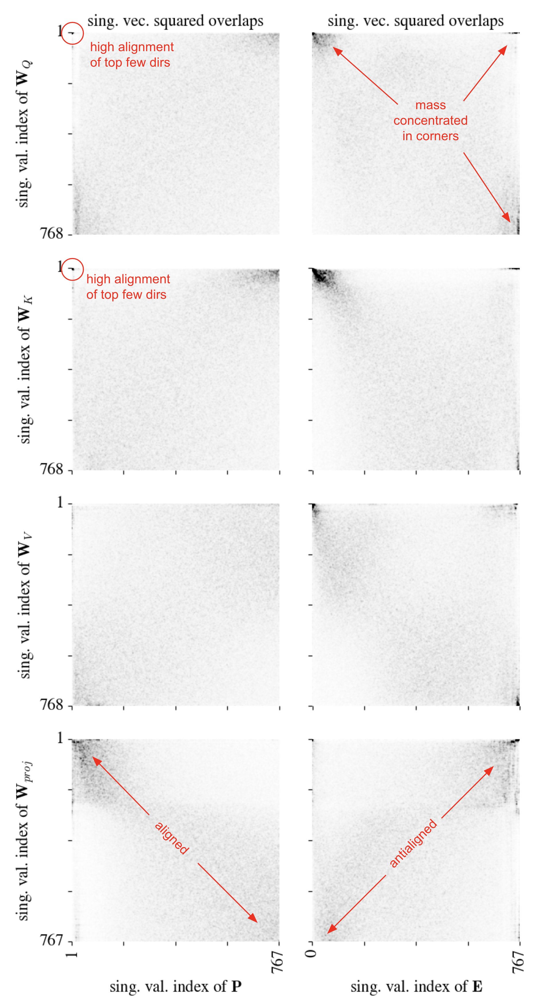
This plot shows that:
- The
queryandkeymatrices are well-aligned to the very top subspace of \(\mathbf{P}\) (note the dark dot in the very top left of the top left two plots – you might have to zoom in). - The
query,key, andvaluematrices are well-aligned to the top subspaces of \(\mathbf{E}\). The corresponding plots have large mass in the top left. - The
projmatrix is well-aligned with \(\mathbf{P}\) and apparently anti-aligned to \(\mathbf{P}\)!
One could come up with various just-so stories here — for example, that the proj matrix is spreading around positional information — but I’ll refrain. The important takeaways are that these matrices are clearly aware of these two important subspaces and that the top few positional encoding directions are used quite a lot in the query-key similary computation, which makes sense. These seem like useful things to keep in mind when, for example, trying to reverse-engineer transformer circuitry.
Claim: [MLP weights] $\perp$ [positional encodings]
Here I will present evidence that the fan-out weights of the first-hidden-layer MLP of GPT-2 have learned to be sensitive to the top directions of the token embeddings and insensitive to the top directions of the positional encodings.
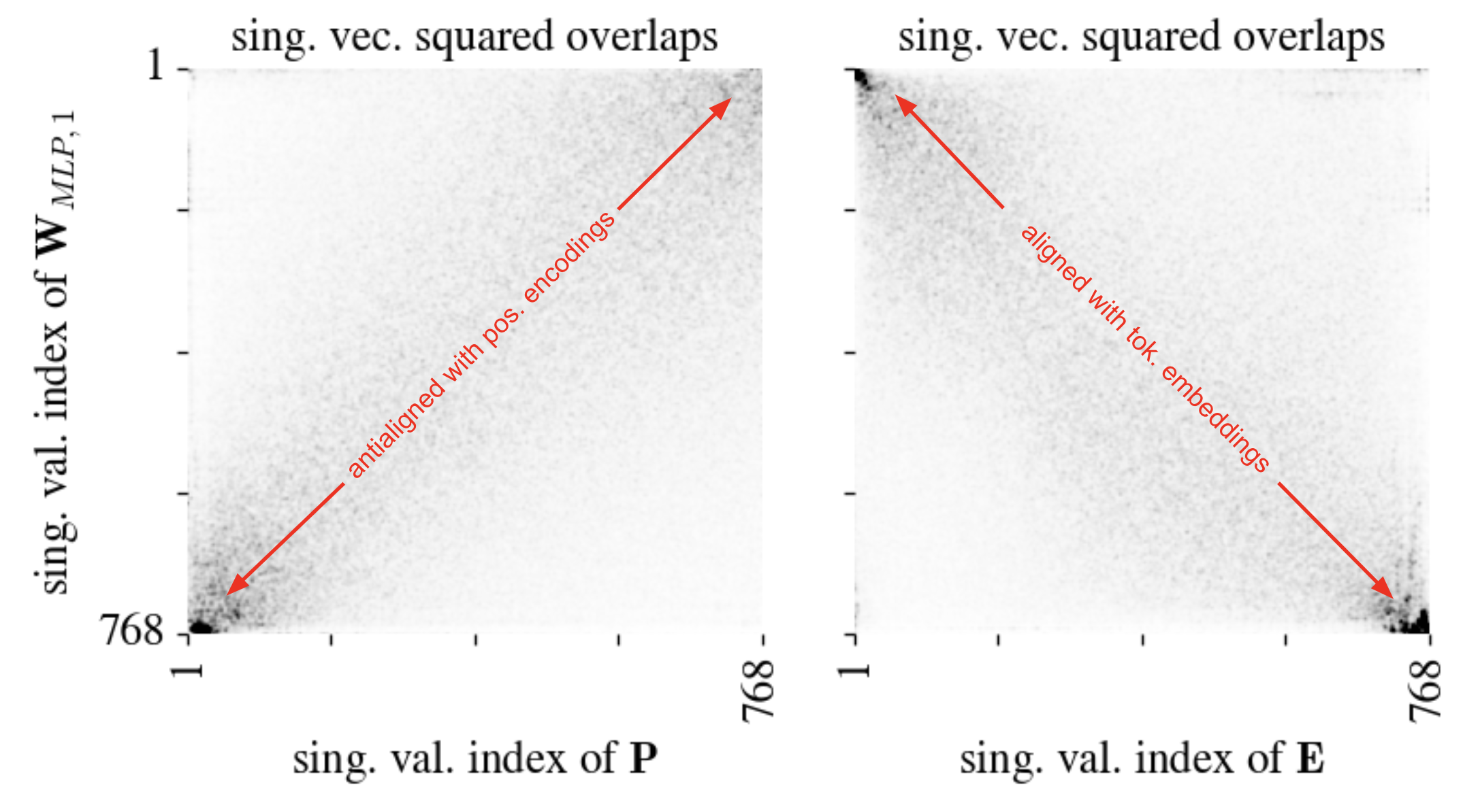
The plot below shows the squared overlaps between the right singular vectors of the MLP weights \(\mathbf{W}_1 \in \mathbb{R}^{d_\text{hid} \times d_\text{model}}\) (with \(d_\text{hid} = 4 d_\text{model}\)) and the positional encoding and token embedding matrices \(\mathbf{P}\) and \(\mathbf{E}\). We see that the MLP is strongly attuned to the top token embedding directions (the first heatmap has most of its mass along the diagonal) and strongly insensitive to the positional encoding directions (the second heatmap has most of its mass along the antidiagonal). This makes sense: the MLP basically acts the same on each token embedding, independently of its position in the sequence.
Claim: the positional encoding subspace is sparse!
Since the top singular subspace of \(\mathbf{P}\) seems to be important, I decided to visualize it. To my surprise, it’s sparse in the embedding space!
Recall that \(\mathbf{P}\) has shape \([d_\text{context} \times d_\text{model}]\), with \(d_\text{context} = 1024\) and \(d_\text{model} = 784\). Let us visualize its top five singular vectors of \(\mathbf{P}\) in these two spaces. The left singular vectors live in the context space, and the right singular vectors live in the embedding space.
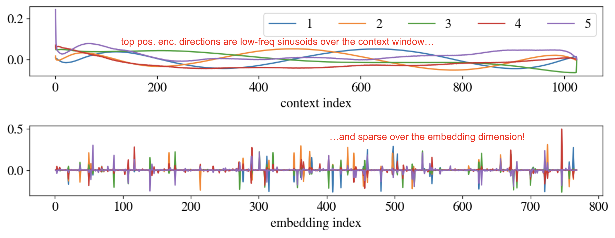
As we might guess, the top singular vectors in the context (i.e. token) space are basically sinusoids of different frequencies… but the top singular vectors in the embedding space are sparse, concentrating strongly on maybe 40 indices. Returning to our original motivation of understanding how the positional encodings don’t interfere with the token embeddings, it seems that not only do they lie in orthogonal subspaces, they actually make use of (roughly) disjoint sets of embedding indices! This is just a permutation away from the positional encodings being appended to the token embeddings rather than added, which makes a lot of sense.
That said, I have no idea why we get sparsification here. I don’t know what induces it; I don’t know why the model prefers this over merely orthogonal subspaces. Odd! It’s a strong enough effect that I’d bet there’s a simple explanation.
Summary
This blogpost describes some purposeful poking around the singular value structure of GPT-2’s positional encoding and token embedding matrices. The main observation – that the these two types of information lie in basically orthogonal subspaces, and this is reflected in intuitive ways in downstream weight matrices – seems pretty solid! There are a bunch of auxiliary observations, including the sparsity of the positional encodings, that seem pretty clear but which I don’t have a good explanation for. In any case, it seems useful to compile heuristic, broad-strokes observations like this when trying to build intuition for how transformers work. Observations like this feel to me like puzzle pieces, and if we get enough on the table, maybe we can start fitting them together.
Thanks to Chandan Singh for proofreading this post and for the discussion that led to it. A Colab notebook reproducing all experiments is here.
-
Two disclaimers here: first, this was written rather fast and some parts might be unclear, and second, I imagine someone out there already knows this! In either case, feel free to drop me a line. ↩
-
For example, if you don’t choose the vectors carefully, you might find that the word
CATat index3is embedded similarly to the wordAPPLEat index6— or, mathematically, that $E(\text{CAT}) + p_3 \approx E(\text{APPLE}) + p_6$ — making them hard to distinguish. ↩ -
I often bump into the problem of how to best measure or visualize the alignment of two matrices. This very info-dense SV-overlap plot is something I hadn’t tried before. I find it somewhat useful and will probably use it in the future. ↩
-
By this I refer to the “projection matrix” from the output of the attention operation back into the residual stream. This isn’t really a projection in any conventional sense, since it’s square – seems better thought of as simply a linear transformation – but that’s what people call it, so we’ll do so here. ↩