Understanding fractals from iterated maps

In this post, I give some mechanistic intuition for why and how the basins of iterated maps form fractals which I feel is usually missing from academic treatments of the subject.

---

It is a remarkable fact of mathematics that simple dynamical systems can display immensely complex behavior. The poster children of this notion are fractals generated from iterated maps. You have likely seen the Mandelbrot set, the most famous such fractal. Here is a related Julia set which is slightly simpler to define:

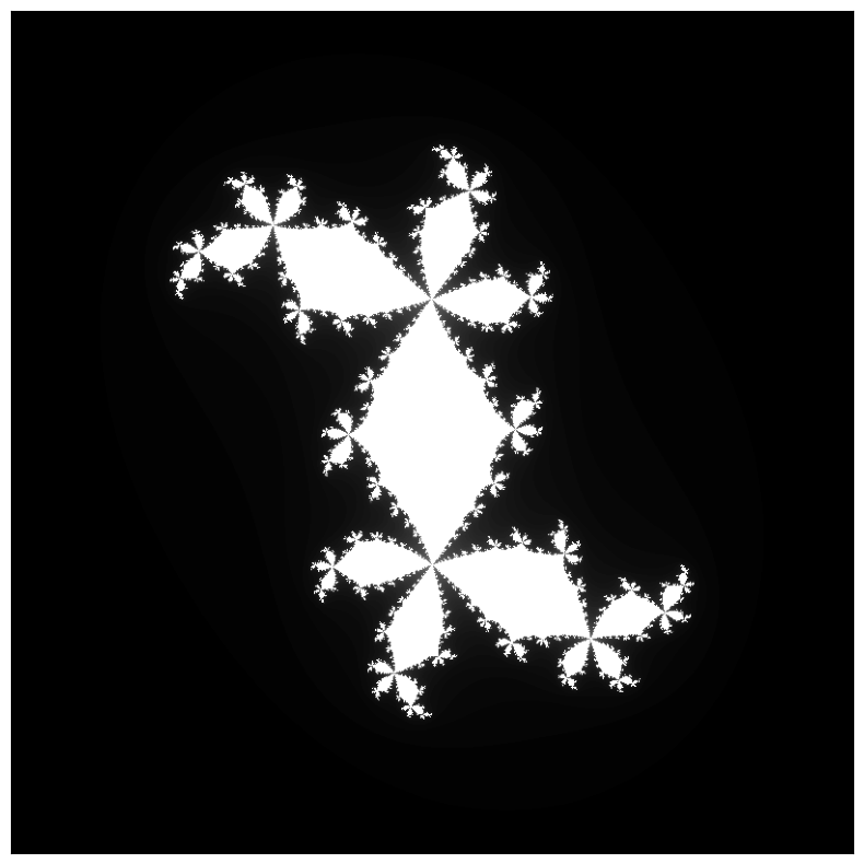
The rule by which this stunning image is generated is remarkably simple. This plot represents the complex plane, and each point \((x, y)\) in the image represents the complex number $z_0 = x + y i$. For each such point $z_0$, we compute $z_1$, $z_2$, and so on using the iterated map

\[z_{t + 1} = f(z_{t+1}) = z_t^2 + c,\]

where \(c \approx 0.2883 + 0.5383 i\) is a parameter I have tuned. This either eventually blows up (with \(|z|\) getting very big) or doesn’t. If $|z|$ blows up, the pixel at $z_0$ is colored white, and if it remains bounded, it is colored black. The result is the stunning fractal above. You can explore different values of $c$ — which generate surprisingly varied and wondrous Julia sets — here.

Where does all this detail come from?

Part of the amazement of images like the above is that our dynamical process was extremely simple to define, but the resulting visualization is quite complicated — infinitely complicated, in fact, or at least infinitely detailed! It gives me (and others, I suspect) the feeling of having somehow “gotten more out than we put in”. It simply does not feel like this dynamical map should be complex enough to generate this fractal!

The answer to this seeming paradox is that we are iterating the dynamical map many times: the level of detail results not from the complexity of the map but rather from the amount of computation we expend repeatedly applying it. This can be beautifully illustrated by visualizing the result of applying only finitely many iterations, using shades of grey to indicate how may iterations a point takes to blow up:

The complexity of these fractals is built up over many iterations.

Why do you get a fractal?

There is a very basic question one can ask here that is virtually never addressed in introductory treatments of chaotic maps:¹ why do we get a fractal? This question is so obvious that, if you’ve already seen this stuff, it’s kind of hard to even see as legitimate: why does the “escape region” of \(f\) take the shape of a fractal? Like, why not some other, non-self-similar shape? Where does the fractal come from? What property of the map $f$ is responsible for the self-similarity?

The usual fact that is given is that these dynamical maps are chaotic. For example, students in a college course might compute the system’s Lyapunov exponent and see that it is positive around the boundary of the fractal, implying the system displays the sensitivity to initial conditions characteristic of chaotic dynamics. Okay, great, it’s believable that these maps are chaotic, but where does this fractal come from? The two concepts are certainly related, but how exactly?

I gnawed on this question sporadically for many years, and I finally have what feels like an intuitive understanding. The main purpose of this blogpost is to convey that (high-level, nonrigorous) intuition. The reason is basically that, if you run the dynamical map forwards, you will find that…

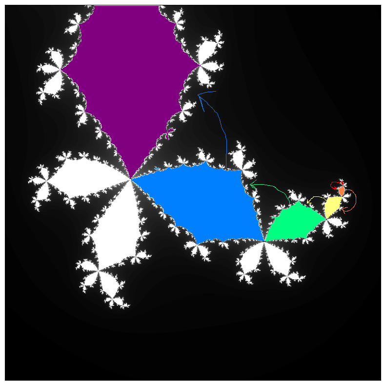
Distinctive regions of the fractal get mapped to larger versions of themselves

This property is easier to show than to tell. Pick a small lobe in the above fractal — say, the little red lobe in the graphic below. If you look around the fractal, you will be able to find lots and lots of little lobes, both bigger and smaller, that have the same shape. Now pick your favorite point in the red lobe. Upon the action of the map $f$, this point will generally be mapped to another point at the same position in a larger version of the same lobe! In the diagram below, an initial point in the red lobe gets mapped to a point in the orange lobe, then the yellow lobe, then the green, and so on.

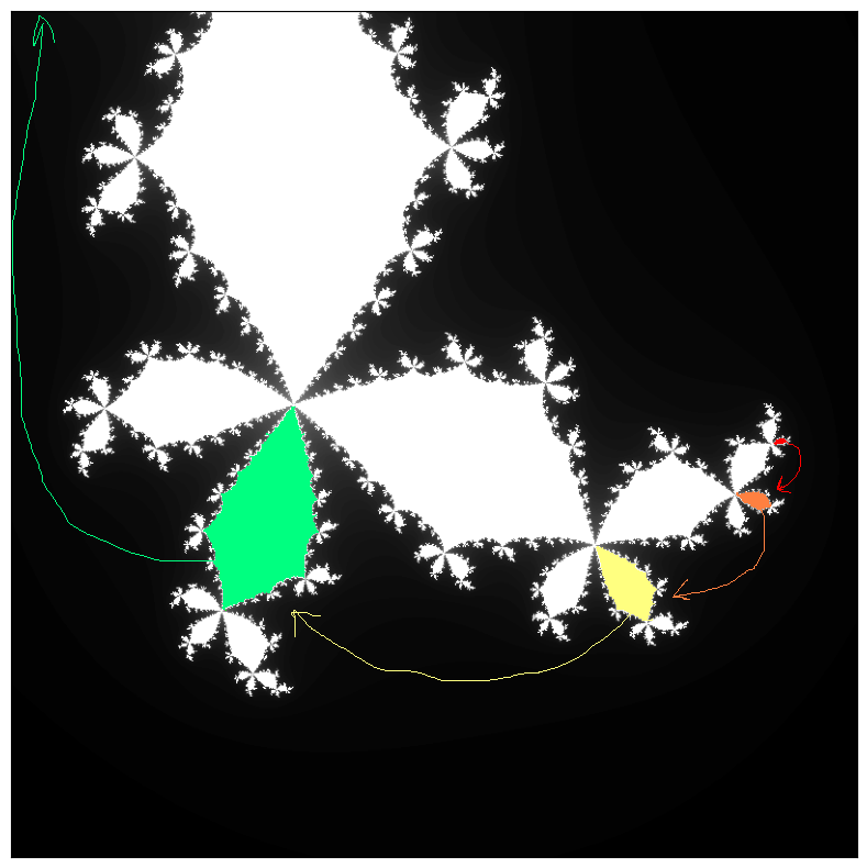
Here’s the same thing with a different starting lobe:

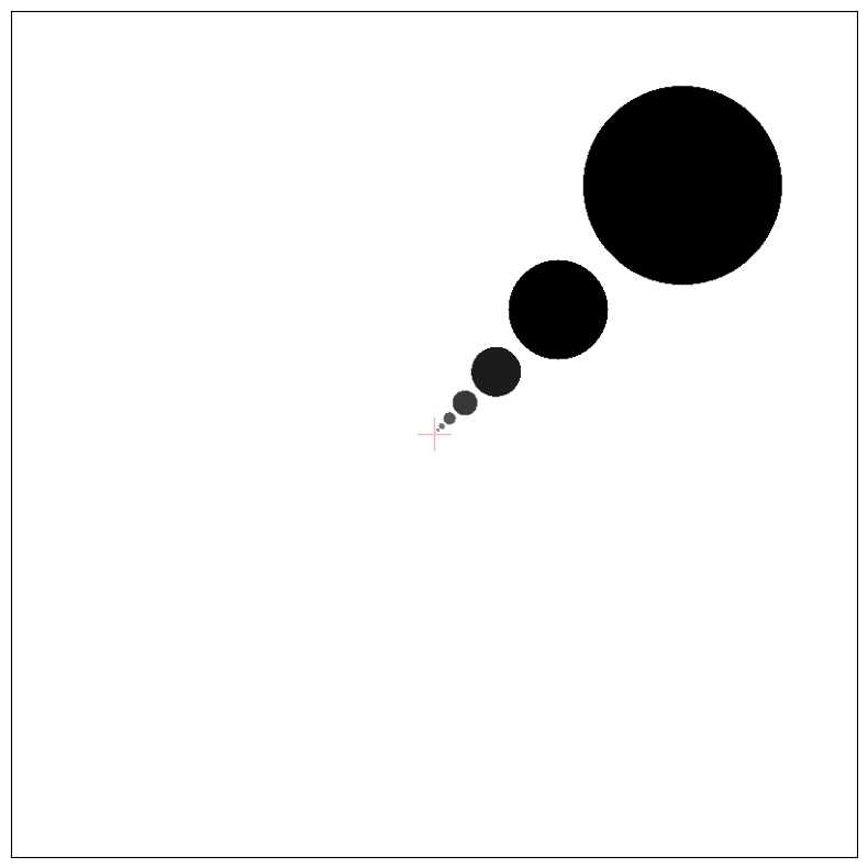
To underscore the first example, here’s an actual computer-generated plot in which the region enclosed by each colored circle is mapped to the region enclosed by the subsequent one:

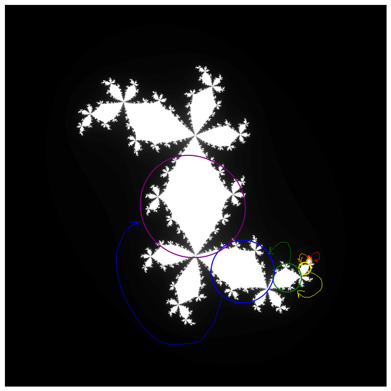
Note how each successive circle here is larger than the one before it, showing that the map is expansive, and the Lyapunov exponents here are positive.

This behavior is enough to explain why the final Julia set contains so many versions of the same lobe. This follows from basically an inductive argument. I will give the argument first and then follow it up with some graphical illustration.

Note first that any point that is mapped to a black point will also be a black point – the two points lie on the same trajectory, so they have the same fate (to diverge or not to diverge). As the base case, assume there is some black region with an interesting shape. As the inductive step, now, suppose that some other, smaller volume of space gets mapped to a volume of space including this black region. There will be a shrunken copy of the black region in this other volume — the black region has been duplicated! Now we can run this process again and again, positing a third, even smaller volume of space that maps to the second, and so on and so on. (Fairly simple mapping functions $f(z)$ can give you an infinite sequence of volumes mapping to each other like this; note that the volumes can overlap. We will give a toy example illustrating this soon.) We now have an infinite number of copies of the original black region, getting ever smaller and more delicate — a fractal!

This really becomes much more tangible when you play around with yourself with an eye to this behavior. You can explore this fractal in-browser at (this nice website)[https://www.marksmath.org/visualization/julia_sets/].

As a final speculation before we use this notion to make some fractals, I wonder if there’s some sense in which getting a fractal is inevitable in the Julia set of a chaotic iterated map. Surely the set will be some chaotic, extremely complicated shape… and it vaguely seems to me like, because the generating function is some fixed function with some finite amount of information required to specify it, it couldn’t possibly result in a chaotic shape which isn’t a fractal — that is, for which each lower level of detail is unlike the higher levels — because that would entail an infinite amount of information to specify. Perhaps there are connections to computational complexity in here, where the function is fixed and has $O(1)$ complexity, but the fractal naively has “geometric complexity” $O(T)$, where $T$ is the number of iterations the map is run for, and somehow the self-similarity of the fractal lets one come up with a new notion of geometric complexity for which these Julia sets only have $O(1)$ complexity. This would feel like a satisfying resolution to the motivating “paradox” that it felt like we were getting more out of these systems than we put in.

Hand-designing some fractals

If you really understand how something works, you should be able to make one yourself. I’m claiming that the ingredients for self-similar basins of attraction from an iterated map are basically (a) expansive behavior and (b) an infinite sequence of volumes that map into each other, leading ultimately to some interesting basin boundary. The easiest way to satisfy both (a) and (b) is perhaps to have some region $\mathcal{R}$ that maps to a larger region $\mathcal{R}’$ that contains both some basin boundary and the original region $\mathcal{R}$ itself. This pretty easily gives an infinite sequence of volumes (and a resulting fractal) because, well, the basin structure within $\mathcal{R}’$ has to contain a complete copy of itself, so self-similar structure is inevitable!

First example: circles in 2D

Here’s an example. We will continue to work in the complex plane and use the map

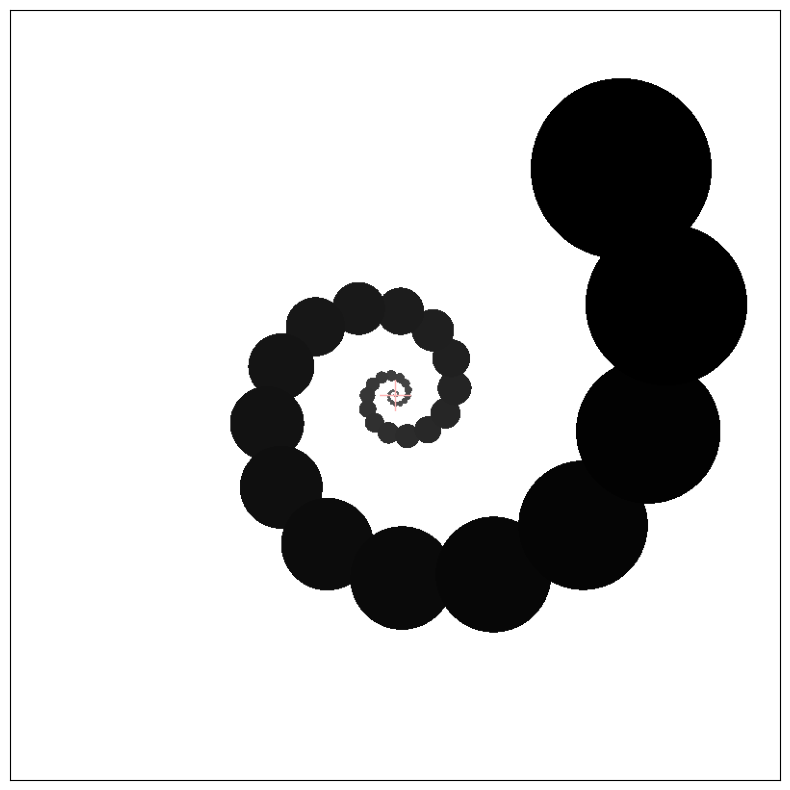
\[z_{t+1} = c z_t,\]

where $c = 2$ for now. I will then draw a circle somewhere in the plane. If a point $z_0$ ever lands inside the circle after some number of iterations, we decree that it may never leave, and we color the pixel at $z_0$ black. If it never lands in the circle, the pixel at $z_0$ is white.

Here’s what you get:

Here I have chosen the “sticky circle” (the largest circle) to have radius $0.4$, centered at $z_c = 1 + i$. The red crosshair shows the origin. Note that we get a fractal!

We can make it more interesting if we instead add some rotation with, say, $c = 1 + 0.1 i$:

Second example: chaotic map in 1D

Let’s design another one. This one will be only 1D. Consider the following map $z_t \mapsto z_{t+1}$:

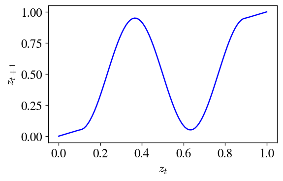
Try to guess what this map will do when iterated many times. It’s not too hard to see that the points on the far left and far right will continue to flow all the way to the edges, so we have $0$ and $1$ as basins of attraction… and I have designed the middle region so that parts of it map into these two basins (the peak and trough), and other parts map back into the whole middle region, guaranteeing that any basin structure is repeated and making the basins structure self-similar. Here’s what this map looks like after being applied seven times:

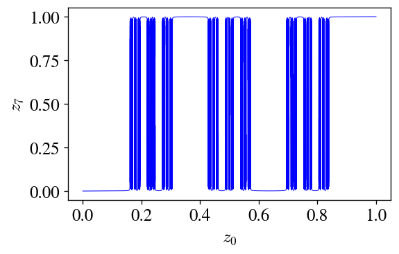
This structure is self-similar (which I verified by zooming in).

Conclusions

In this post, I’ve aimed to give some mechanistic insight into why and how the basins of attraction of iterated maps give fractals. There’s a huge raft of technical content I could have brought in here but didn’t — if you’re interested, I’d encourage you to check out Lyapunov exponents, the logstic map, the Mandelbrot set, and perhaps Steven Strogatz’ Nonlinear Dynamics and Chaos. I had never really felt I could see the genesis of this class of fractals before, but now I can, so I hope this sheds some light for some other folks, too!

A major takeaway I have here, which I didn’t fully appreciate before, is that in systems like these, chaos is usually studied as a local property — e.g., the Lyapunov exponent is positive, and it’s locally defined — but these fractals are global. I think this probably explains why I hadn’t encountered a good explanation like this before: it seems hard to reduce the global property of fractal-formation to a property of the return map that’s simple enough to prove a theorem about. I wonder if there’s some analytical condition on the return map that one could define that’d be necessary and sufficient for it to give you fractals.

---