Geometric patterns in croplands

I’ve lived in California for five years now and have had the good fortune to roam up and down the state and see its mountains, valleys, and deserts. As any outdoorsy Californian will know, these treks often featured long drives through the Central Valley, past wide fields of California crops: fruits, nuts, grain. As a frequent passenger in these drives, I’ve come to look forward to gazing out a changing windowful of cropland, particularly when it makes a certain sort of geometric pattern.

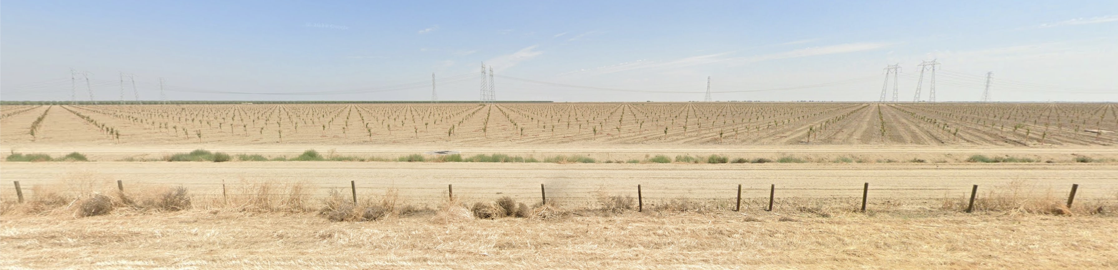
If you’re not familiar with this effect, take a minute to really examine the strip of field planted with the baby trees. As you scan across the strip, you’ll notice places where the saplings form lines leading off into the distance. The lines have different degrees of definition, and the gaps between the lines have different sizes in different places. The “regions” of lines seem to have a curious fractal pattern: if you look between two neighboring line-regions, you’ll find another, smaller set of more closely spaced lines, and so on recursively. I find it mysterious and beautiful. For fun, you can click on the above image to be taken to the corresponding spot in Google Streetview if you want to explore it for yourself.

The regions pop out to the eye even more when you’re moving! Here’s a gif of the view out my window as I drove by the same place.

What’s going on? In this post, I’ll explain why we see these “open” directions and try to explain why the overall visual effect is so fractally. The basic explanation of the open regions will need only some simple math used in the physics of crystals. When we try to understand the fractally effect, we’ll encounter some cool number theory. I’ll end with a neat numerical experiment and an open question.

The open directions of an infinite lattice

The nature of the special directions is easily understood starting from the observation that these saplings are planted in a near-perfect rectangular grid.¹ In such a grid, one expects the plants to leave “aisles” along the grid directions, and if one plays around with a drawing of a grid, one soon observes that the points also form narrower isles in other, off-axis directions. See the colored “aisles” in the illustration below.

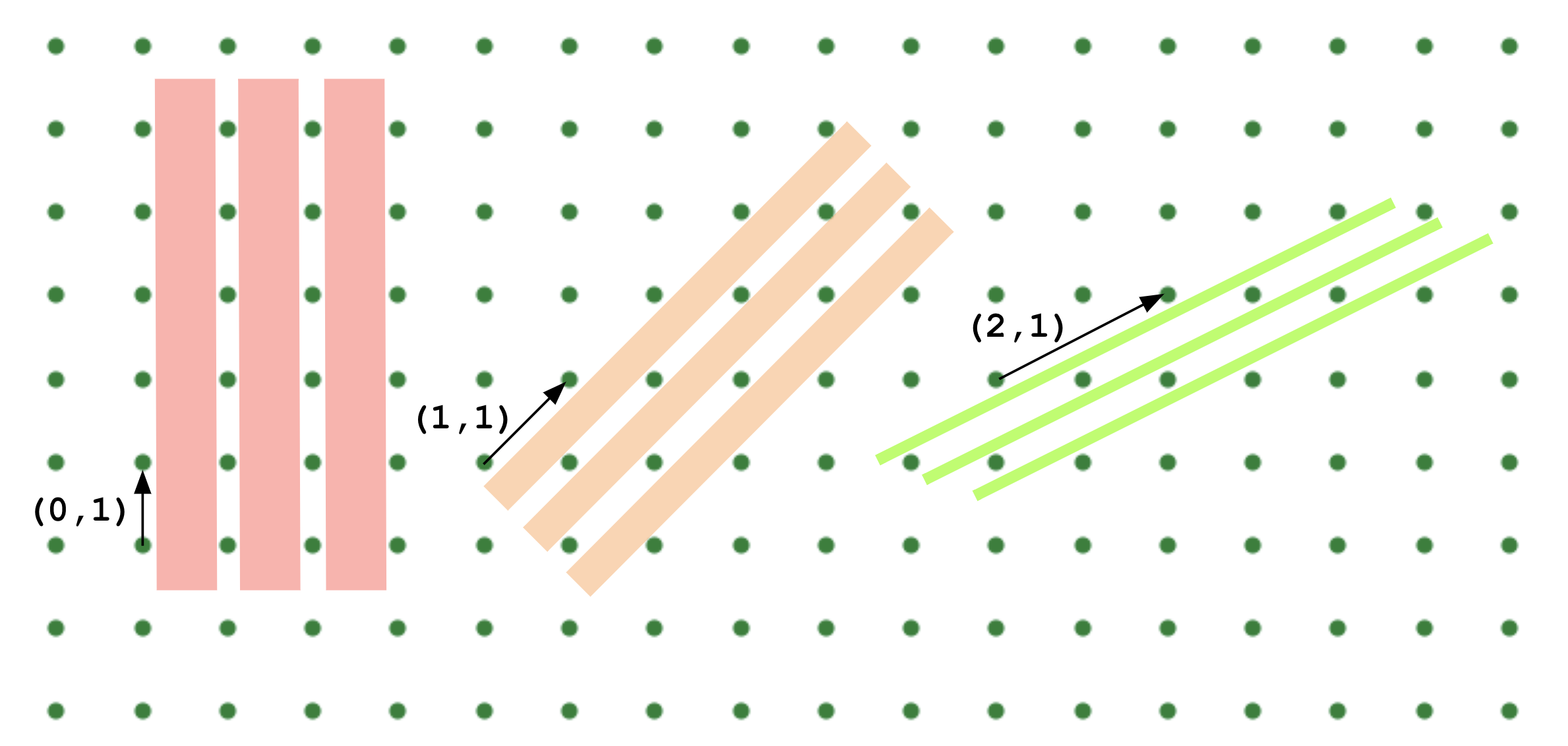
The three examples in the above illustration correspond to particular “lattice vector” – that is, vectors \((a, b)\) with integer components, with \(a, b\) “irreducible” – that is, sharing no factors greater than \(1\).² It turns out that all “open directions” – that is, directions one can look without hitting (or passing arbitrarily close to) a tree – correspond to such lattice vector!

The above illustration highlights the gaps between the rows of trees, but we might similarly talk about the rows of trees lying between the colored rectangles. This is the perspective taken in crystallography. The atoms in a crystal form a regular lattice by definition, and this lattice can be decomposed into many parallel rows (or sheets in 3D), and light of the appropriate frequency will scatter off these surfaces as if they were partially reflective mirrors. This is a common experimental technique for identifying different crystals.

Which open directions will you see?

Great – we now have a rule describing our open directions: every direction in which one can gaze unblocked off to infinity is parallel to a lattice vector \((a, b)\), where \(a, b\) are an irreducible pair of integers. When we look out at a big field, we should thus see a total number of… *furiously counting on fingers* infinitely many open directions, one for every \((a, b)\). Well, that doesn’t seem right, looking at our photograph above – what’s gone wrong?

Three things. First, the field in the photo above is finite, and there are some directions we don’t see that would emerge if the field were extended. Second, our camera has finite resolution. Third, the trees have nonzero width – some lattice directions give wider “aisles” than others, and if an aisle’s narrower than the size of a tree, we won’t see it even provided an infinite field and perfect camera.³

All three of these effects point to a general conclusion: wider “aisles” are more visually salient. It’d thus be useful to know the “aisle width” (or equivalent the “lattice row spacing”) corresponding to a particular lattice direction. Some quick geometry tells us that, with pointlike trees on a unit lattice, the aisle width in direction \((a, b)\) is \(w_{a,b} = \frac{1}{\sqrt{a^2 + b^2}}.\) This gives us a satisfying ordering of lattice directions: a lattice direction \((a, b)\) is more visually salient the smaller \(\sqrt{a^2 + b^2}\) is – that is, the closer it is to the origin! We should thus expect the directions \((0, \pm 1)\) and \((\pm 1, 0)\) to appear most visually striking, followed by \((\pm 1, \pm 1)\), then \((\pm 1, \pm 2)\) and \((\pm 2, \pm 1)\), and so on and so forth.

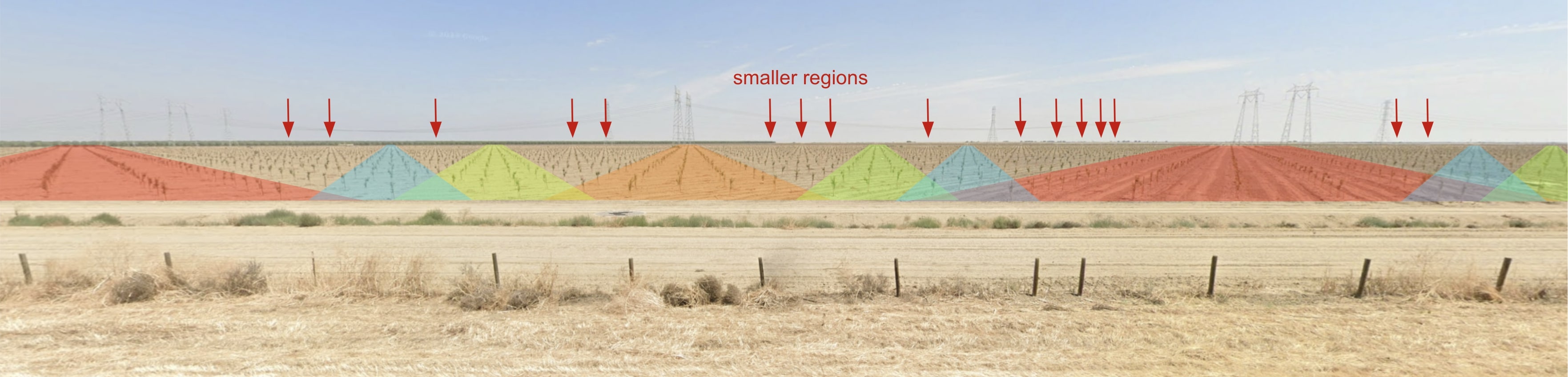
I’ve annotated our original image with the actual lattice directions. This is precisely what we see:

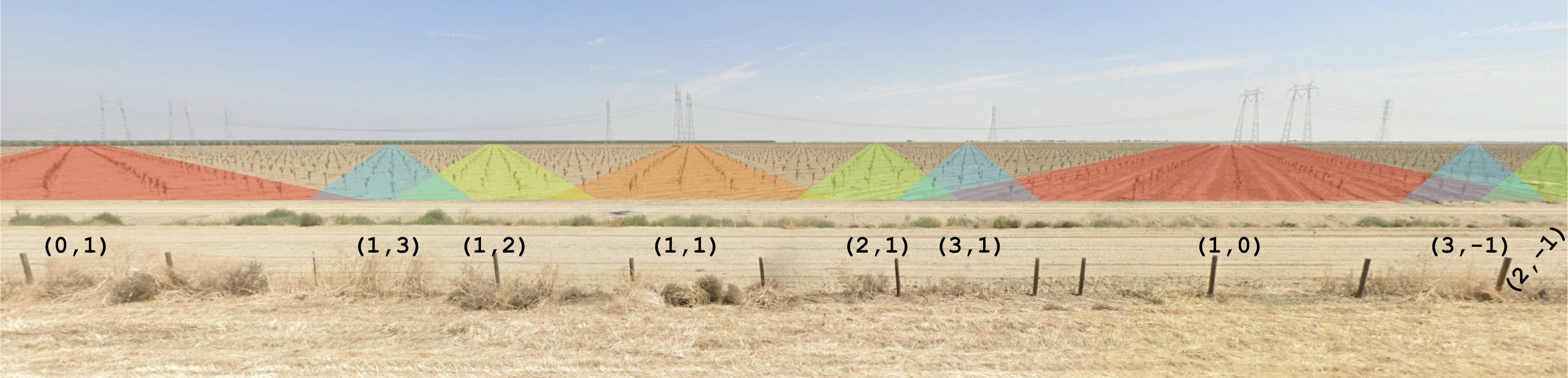
If we had an infinite field and a camera of good enough precision, we’d expect to see open directions corresponding to all irreducible \((a, b)\) such that \(w_{a, b} < d\).

Fancy math: Farey sequences and recursive structure

The math so far is pretty familiar to physicists – we’re used to thinking about lattices and lattice vectors, having seen them a hundred times in quantum courses. As I’ve looked out at scenes like this, the thing I really wanted to understand is: why does it look so fractal?

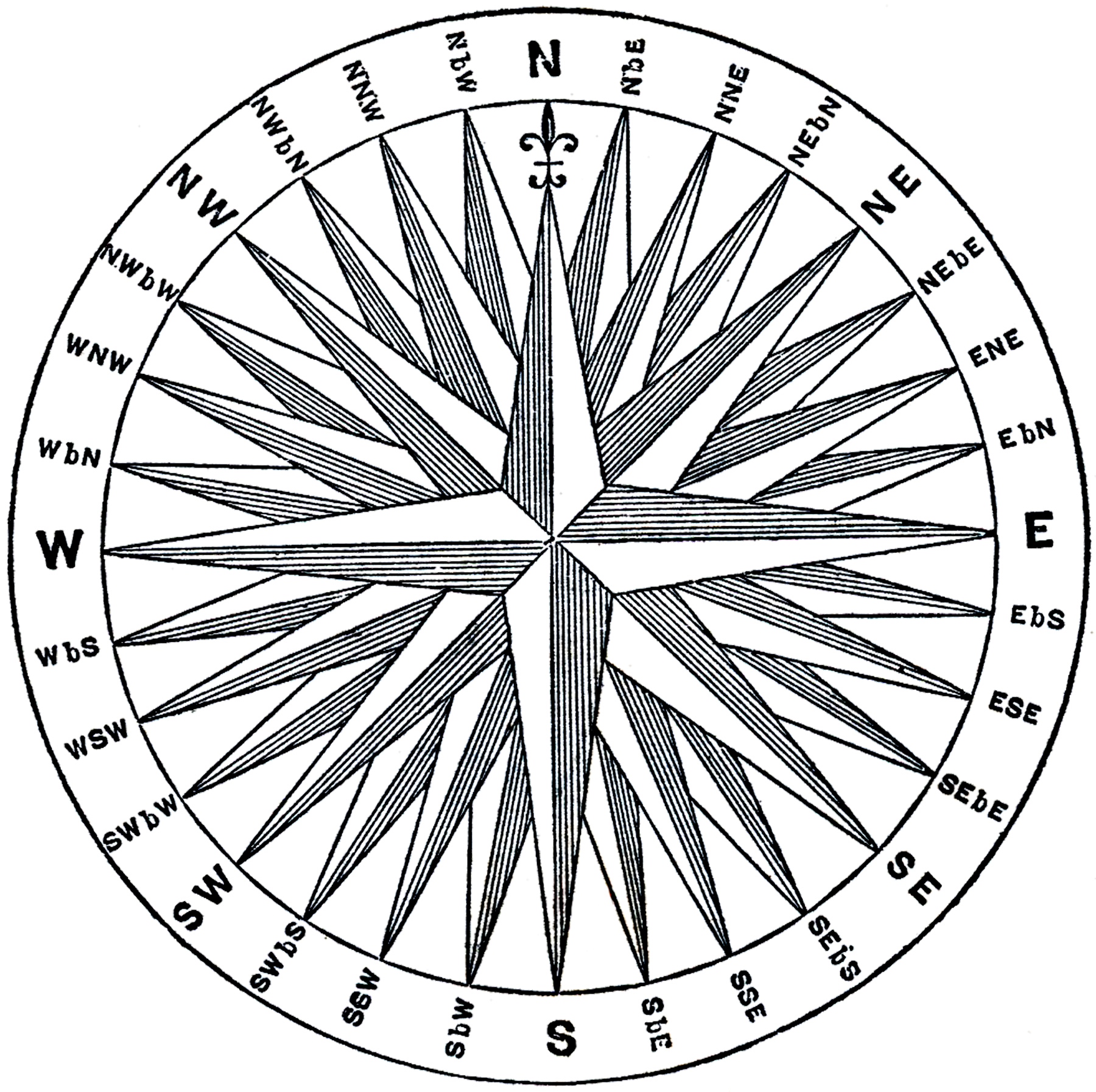
Let me try to be more precise: the little triangles of open “aisles” in our field photograph sure give the impression of a sort of recursive structure – given two big triangles, one usually finds a medium triangle between them, and there are never two big triangles too close to each other, sort of like a compass rose:

It very much looks to me like, if you started adding triangular regions in order of decreasing size, you’d tend to insert each new triangle closer than chance to the midpoint of its neighbors. I actually simulated this and it’s not true – to my surprise the distribution appears to be uniform – but in my trying to understand this I did come across some cool math.

Farey sequences are sequences of rational fractions defined in the following manner: the Farey sequence of order \(n\) consists of all unique rational numbers in \([0,1]\) with denominator less than or equal to \(n\). This actually maps nicely onto our problem restricted such that \(b \ge a \ge 0\), in which case the valid \(\frac{a}{b}\) are exactly the rational numbers in \([0, 1]\). The Farey sequences have many weird properties, one of which is the following: if \(\frac{a}{b}\) and \(\frac{c}{d}\) are neighbors in a Farey sequence, then as you increase \(n\), the first element to appear between them is always \(\frac{a + c}{b + d}\). In our problem, that means that if there are open directions at \((a, b)\) and \((c, d)\) and no bigger open direction between them, then the biggest open direction between them will lie at \((a + c, b + d)\)! For example, the biggest open direction between \((0,1)\) and \((1,0)\) is \((1,1)\), and the biggest open direction between Farey-neighbors \((3,5)\) and \((2,3)\) is \((5, 8)\). The wiki page for the Farey sequences has all sorts of interesting recursive diagrams that fall out of this recursive structure. (Sidebar: as of writing, I don’t understand why this property is true. I’d be happy to have someone explain it to me!)

What does this tell us about the visual effect one sees when looking out at a regularly-planted field? Well, it means that, when adding the next-biggest open region between two existing regions, it’ll tend to be placed closer to the smaller of the two existing regions. Looking back at our field photograph (esp the version annotated with arrows), this is certainly the case!

Can “apparent openness” vs. angle be described by a smooth function?

Number theory is very beautiful, but essentially discrete in nature. The special directions we find are pointlike: look in one particular direction and you’ll see forever, but a little bit to either side and you won’t. However, when I look out at a cropfield like this – particularly at the gif – my eye isn’t just drawn to certain points: a bigger region leading up to the point at infinity pops out to me visually. This makes sense – in the idealized setting, if I look slightly off an infinite-sight direction, I’ll still see pretty far! This makes me want some kind of continuous function of angle that tells me, say, how far I’ll typically see when looking in that direction. Perhaps this function is parameterized by some notion of tree diameter \(d\), and has peaks that appear at the rational angles as \(d\) decreases.

I’ll say upfront that I tried for a while and didn’t come up with anything nice. This is the open question: can one write down a nice analytical function of angle that in some sense captures “how far” one can see along angle \(\theta\) through a forest of regularly-spaced trees of diameter \(d\)?

What I do have is a hacky numerical experiment and some cool plots. I’ll use a proxy metric I can compute in Python: with trees of diameter \(d\), what’s the farthest one could possibly see in direction \(\theta\) if one stood in the optimal place? Well, actually, I’ll use a metric that’s almost the same (in particular being infinite in the same places) but easier to compute: with pointlike trees, what’s the longest rectangle of width \(d\) that one can fit anywhere in the lattice with long side at angle \(\theta\) from an axis?

Here’s a gif of the result.⁴

There’s a lot of cool stuff to see in this! Most obviously, you can see the lattice directions opening up in the predicted sequence: the cardinal directions (\((1,0)\) etc.) are open at the start, and then the \((1,1)\) direction and friends open up when \(d = \frac{1}{\sqrt{2}}\), and then the \((1,2)\) directions and friends open up, and so on. Interestingly, a direction is always a local minimum just before it opens up – when \(d\) is just larger than \(w_{a,b}\), changing angle just a little bit in either direction will let you “see” one tree further. This is a neat one to try to understand by playing with a diagram yourself. There also seem to be no local maxima that aren’t vertical asymptotes. These properties give the process a sort of fractally feel: concave-up regions between vertical asymptotes get recursively split in two by new asymptotes.

This is cool and all – it’s a parameterized function which gains vertical asymptotes corresponding to all the rational numbers as the parameter decreases! – but I still want a nice analytical version of this. If you have any ideas, let me know!

Code and acknowledgements

You can find my code for generating these plots here. Thanks to Vincent Huang for pointing me to Farey sequences.

---