Infinite-width autoencoders are cursed
In this blogpost, I show that infinite-width neural networks with a finite-width layer in the middle are cursed: they can’t be parameterized so that, when trained with gradient descent, they (a) train in finite time and (b) have their weight tensors undergo alignment as prescribed by $\mu$P. I conclude by describing two modifications that fix this problem.
Autoencoder? I hardly know her!
~ Traditional San Francisco saying
How do you width-scale an autoencoder?
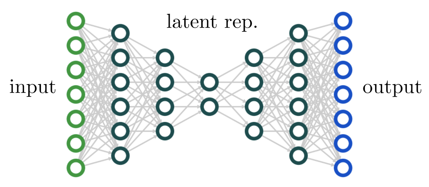
Autoencoders are neural networks designed to extract (comparatively) low-dimensional representations from high-dimensional data. They’re widely-used tools for dimensionality reduction, and in the form of VAEs, data generation. The classic autoencoder design looks like an hourglass: the input layer is the widest, subsequent layers have fewer and fewer layers until they reach a narrowest “bottleneck” layer, and then the sequence is repeated in reverse.
An autoencoder is usually trained with a reconstruction objective — that is, with the goal of learning the identity function $f: x \mapsto x$ on the data.
Autoencoders are interesting from a scaling perspective because they represent a case where finite width is desirable, at least in one layer. They won’t learn interesting representations if every hidden layer is wide. That said, a predominant lesson from the last few years of deep learning is that, insofar as network architecture is concerned, wider is always better so long as your hyperparameters are properly tuned. In what sense will this also be true of autoencoders?
Asked from another direction: how should you take the large-width limit of an autoencoder? Which layers in the hourglass above do you take to be infinite width? All of them except the input, bottleneck, and output? Do you preserve the hourglass taper, jumping up to a large width $N$ at the second layer but then gradually decreasing width down to a constant-width bottleneck? If so, do you taper width down by a constant factor $C$ per layer so the width at layer $\ell$ is $C^{-\ell}N$? Do you take widths $N^{-\alpha(\ell)}$ with $\alpha(\ell)$ interpolating from $1 \rightarrow 0$? It’s unclear!
In this blogpost, I will show that the answer is that, with the standard notion of neural network parameterization, you cannot. There is no consistent way to take an infinite-width limit such that the net satisfies typical notions of layer alignment and feature learning. I’ll demonstrate this by examining a two-layer slice of a deep net, aiming to convey the general problem by means of this example. I’ll then give some solutions.
Example: a width-one bottleneck
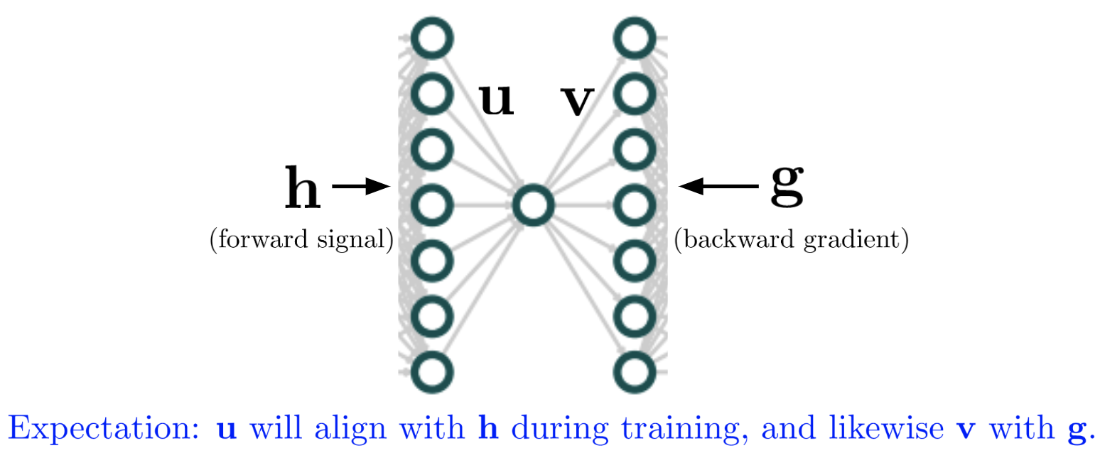
Consider a deep network which has hidden width $n_k = N$ at most layers but one bottleneck layer $\ell$ with width $n_\ell = 1$. Suppose there is no nonlinearity at the bottleneck layer or adjacent layers. For the weights before and after the bottleneck, let us adopt the shorthand $\mathbf{u}^\top = \mathbf{W}_{\ell-1}$ and $\mathbf{v} = \mathbf{W}_\ell$, with $\mathbf{u}, \mathbf{v} \in \mathbb{R}^N$. Let us write $\mathbf{M} = \mathbf{v}\mathbf{u}^\top \in \mathbb{R}^{N \times N}$ for the full rank-one parameter block comprised of these two weight matrices.
We will consider training these two weight matrices through several steps of SGD on a single example $x$. Let us denote the hidden vector passed into this bottleneck block by $\mathbf{h} = \mathbf{h}(x) \in \mathbb{R}^N$, denote the output of the block by $\tilde{\mathbf{h}} = \tilde{\mathbf{h}}(x) \in \mathbb{R}^N$, and denote the gradient backpropagated into this block by $\mathbf{g} = -\nabla_{\tilde{\mathbf{h}}} \mathcal{L}$, where $\mathcal{L}$ is our global loss. We will assume for simplicity that $\mathbf{h}$ and $\mathbf{g}$ do not change for these steps. Note that the parameter gradient applied to the whole matrix is $\nabla_\mathbf{M} \mathcal{L} = \mathbf{g} \mathbf{h}^\top$. The following figure illustrates our notation:
Key feature learning desideratum: weight alignment
Suppose that we have just randomly initialized the parameters $\mathbf{u}, \mathbf{v}$ and will proceed to train for several steps with fixed learning rates. Let us denote the alignment between the weight vectors and their corresponding signal vectors by
\[\mathcal{A}_{\text{in}} = \frac{\mathbf{u}^\top \mathbf{h}}{|\!| \mathbf{u} |\!| |\!| \mathbf{h} |\!|}, \quad \mathcal{A}_{\text{out}} = \frac{\mathbf{v}^\top \mathbf{g}}{|\!| \mathbf{v} |\!| |\!| \mathbf{g} |\!|}.\]At initialization, when $\mathbf{u}, \mathbf{v}$ are random vectors, we have that $\mathcal{A}_\text{in}, \mathcal{A}_\text{out} = \Theta(N^{-1/2})$.
Under the precepts of $\mu$P, we desire the following two natural conditions of feature learning:
Weight alignment desideratum. After $O(1)$ steps of training, we desire that $\mathcal{A}_\text{in}, \mathcal{A}_\text{out} = \Theta(1)$.
No-blowup desideratum. After a handful of steps of training, the norms of each weight matrix should have reached their final size, scaling wise. That is, $\frac{|\!| \mathbf{u}_{t+1} |\!|}{|\!| \mathbf{u}_t |\!|} = \Theta(1)$ and likewise for $\mathbf{v}$.
The first desideratum captures the intuitive notion that weight matrices should align to (the top singular directions of) their gradients upon proper feature learning. In conventional parlance, feature evolution is about leading-order change in the activations, not the weight tensors, but these are in fact two sides of the same coin, as one finds upon a spectral-norm analysis of deep learning. The second desideratum basically says that we don’t want things to blow up. Obviously, if we take infinite learning rates, these matrices will align just fine, but their norms won’t stabilize. It’s fine to initialize one of them to be very close to zero, but its norm should stabilize after a few steps.
We’ll now see that these intuitive desiderata are incompatible for training under SGD.
Evolution under SGD
Suppose we have learning rates $\eta_u$ and $\eta_v$ for $\mathbf{u},\mathbf{v}$, respectively. These vectors then see gradient updates
\[\delta \mathbf{u} = \eta_u \cdot \mathcal{A}_\text{out} \cdot |\!|\mathbf{h}|\!| |\!|\mathbf{g}|\!| |\!|\mathbf{v}|\!| \cdot \hat{\mathbf{h}},\] \[\delta \mathbf{v} = \eta_v \cdot \mathcal{A}_\text{in} \cdot |\!|\mathbf{h}|\!| |\!|\mathbf{g}|\!| |\!|\mathbf{u}|\!| \cdot \hat{\mathbf{g}},\]where $\hat{\mathbf{h}}, \hat{\mathbf{g}}$ are unit vectors in the directions of $\mathbf{h}, \mathbf{g}$. We are free to absorb $|\!| \mathbf{h} |\!|$ and $|\!| \mathbf{g} |\!|$ into the definitions of $\eta_u, \eta_v$. More subtly, we are free to absorb the initial scales of $|\!| \mathbf{u}_0 |\!|$ and $|\!| \mathbf{v}_0 |\!|$ into the learning rates, too, and so will henceforth assume that these vectors are of the same size up to a constant factor.1
\[\delta \mathbf{u} = \tilde \eta_u \cdot \mathcal{A}_\text{out} \cdot |\!|\mathbf{v}|\!| \cdot \hat{\mathbf{h}},\] \[\delta \mathbf{v} = \tilde \eta_v \cdot \mathcal{A}_\text{in} \cdot |\!|\mathbf{u}|\!| \cdot \hat{\mathbf{g}}.\]From this, we may assess the update norms as
\[\frac{|\!| \delta \mathbf{u} |\!|}{|\!| \mathbf{u} |\!|} = \tilde \eta_u \cdot \mathcal{A}_\text{out} \cdot \frac{|\!| \mathbf{v} |\!|}{|\!| \mathbf{u} |\!|} \sim \tilde \eta_u \cdot \mathcal{A}_\text{out},\] \[\frac{|\!| \delta \mathbf{v} |\!|}{|\!| \mathbf{v} |\!|} = \tilde \eta_v \cdot \mathcal{A}_\text{in} \cdot \frac{|\!| \mathbf{u} |\!|}{|\!| \mathbf{v} |\!|} \sim \tilde \eta_v \cdot \mathcal{A}_\text{in},\]where we have made use of the fact that $\frac{|\!| \mathbf{v} |\!|}{|\!| \mathbf{u} |\!|} = \Theta(1)$. We now return to our boxed desiderata. To satisfy the weight alignment desideratum, we require $\frac{|\!| \delta \mathbf{u} |\!|}{|\!| \mathbf{u} |\!|} = \Omega(1)$ and likewise for $\mathbf{v}$. To satisfy the no-blowup desideratum, we require $\frac{|\!| \delta \mathbf{u} |\!|}{|\!| \mathbf{u} |\!|} = O(1)$ and likewise for $\mathbf{v}$. Combining both, we find that $\frac{|\!| \delta \mathbf{u} |\!|}{|\!| \mathbf{u} |\!|} = \Theta(1)$ and likewise for $\mathbf{v}$.
We may now observe a contradiction. After a few steps we will have that $\mathcal{A}_\text{in}, \mathcal{A}_\text{out} = \Theta(1)$, from which we may conclude that $\tilde \eta_u, \tilde \eta_v = \Theta(1)$. However, these learning rates are too small to cause alignment to begin with! At early times when the alignments are near zero, we have
\[\frac{d}{dt} \mathcal{A}_\text{in} \sim \tilde{\eta}_u \cdot \mathcal{A}_\text{out} \sim \mathcal{A}_\text{out},\] \[\frac{d}{dt} \mathcal{A}_\text{out} \sim \tilde{\eta}_u \cdot \mathcal{A}_\text{in} \sim \mathcal{A}_\text{in}.\]Treating “$\sim$” as “$=$,” the solution to this coupled ODE from small initial value is
\[\begin{bmatrix} \mathcal{A}_\text{in} \\ \mathcal{A}_\text{out} \end{bmatrix} \approx e^t \begin{bmatrix} \mathcal{A}_0 \\ \mathcal{A}_0 \end{bmatrix},\]where $\mathcal{A}_0 = \frac{1}{2} [\mathcal{A}_\text{in} + \mathcal{A}_\text{out} ]_{t=0}$ is the average of the initial alignments. We can now observe that, in order to grow to order unity from an initial size of $\Theta(N^{-1/2})$ requires a number of steps $T$ such that $e^T N^{-1/2} = \Theta(1)$, which implies that $T \sim \log N$! As $N$ grows, it takes longer and more and more steps to reach alignment.
What, intuitively, is going on?
The crux of the problem here is that each weight tensor’s gradient is mediated by the other weight tensor’s alignment. The more aligned one tensor is, the bigger an update the other one will see. The problem is that since both alignments start small, the dynamics are a classic case of two small variables suppressing each other’s gradients!2 We’re stuck with a Catch-22: we could jack up the learning rates to have huge updates at the start that overcome the tiny init, but then our dynamics at late times blow up! However, if the learning rate is small enough so the dynamics at late time don’t blow up, then the dynamics take a long time to get going.3
A simulation
Below is a sweep of SGD trajectories for the loss $\mathcal{L} = (\mathbf{h}^\top \mathbf{u} \mathbf{v}^\top \mathbf{g} - 1)^2$. I have taken $|\!| \mathbf{h} |\!| = |\!| \mathbf{g} |\!| = 1$ and initialized with $u_i, v_i \sim N^{-1/2}$, because any larger init will not have aligned at convergence, and any smaller init will still suffer from the core problem but worse. I train both vectors with a learning rate $\eta$ and vary $N$. I train for a fixed number of steps $T = 10$.
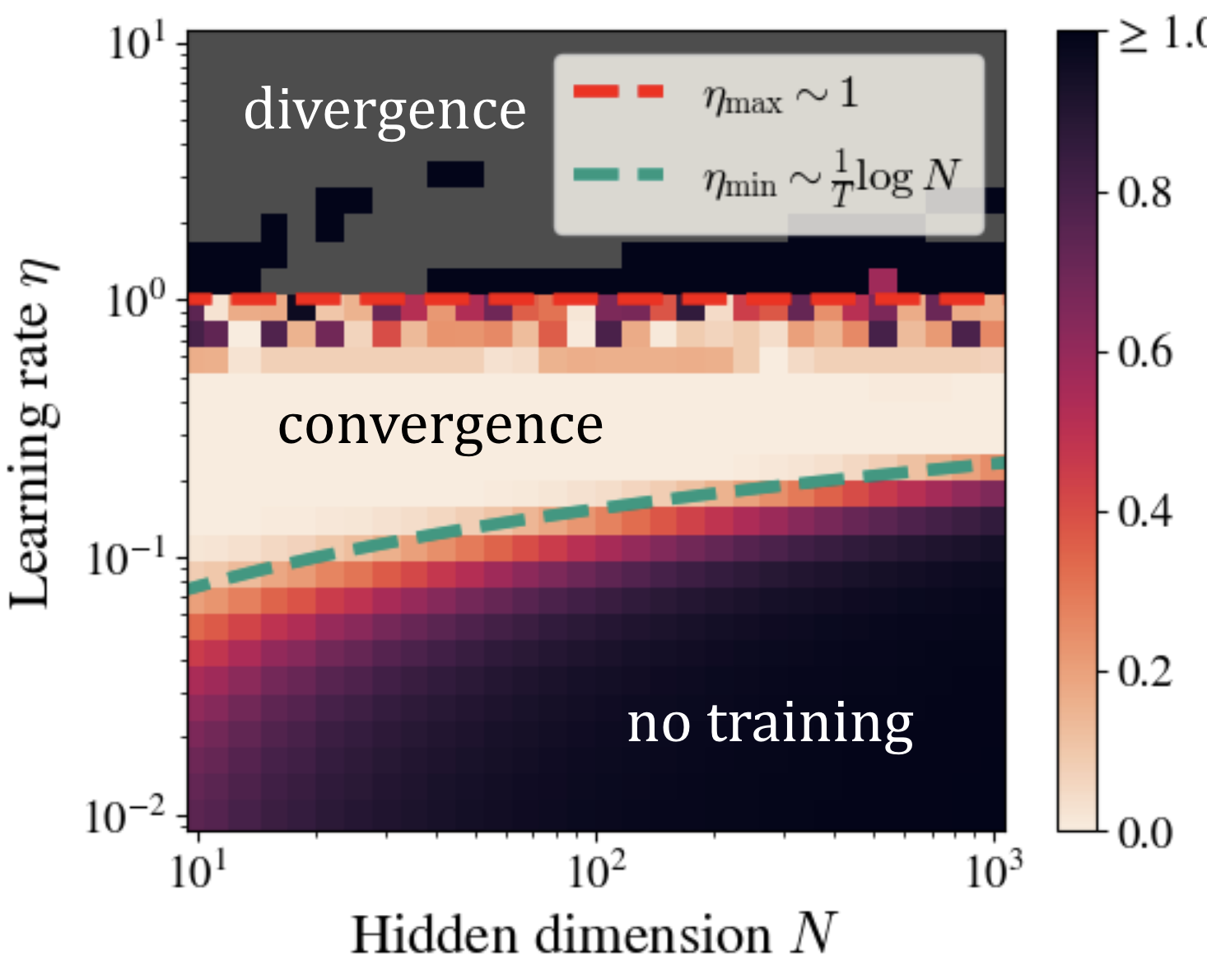
One can clearly see that the region of optimizability is shrinking, albeit slowly, with $\eta_\text{min} \sim \log N$ and $\eta_\text{max} \sim 1$ bound to converge at sufficiently large $N.$ A Colab notebook reproducing this experiment may be found here.
So what? Requiring $\log N$ time isn’t so bad.
That’s true. The two reasons to care are that:
- In our theoretical models, we want to work at truly infinite width, and the logarithmic factor still blows up.
- Hyperparameter transfer ($\mu$Transfer) probably won’t work because the infinite-width process isn’t well-defined.
So there you have it. Infinite-width networks with finite-width bottlenecks are cursed and can’t be trained in a traditional fashion so all layers align to their gradients. The above argument can be extended to bottlenecks with finite width $k > 1$, and even to those with any width $k = o(N)$, though that’d require some random matrix theory to see.
This was actually an awkward point that came up during the writing of “A Spectral Condition for Feature Learning.” We never resolved it, we just didn’t discuss it! It’s fine for most architectures, but it does feel like a lingering problem with $\mu$P. What is to be done?
Two possible solutions: rank regularization and cascading init
Here I’ll pitch two solutions that I think can be used to width-scale autoencoders.
The first is to ditch the variation in width between layers — just keep everything width-$N$ — and instead enforce the rank constraints implicitly with regularization. For example, if a layer is intended to have fan-out dimension $k$, one could gradually turn on an $\ell_1$ regularization on all but the top $k$ singular vectors of the weight matrix until the regularization is so high that it becomes sparse. I believe this is consistent even at infinite width, though it does unfortunately require computing the SVD lots of times.
The second idea is to do a “cascading init” in the following fashion. First, initialize all weight tensors to zero. Next, choose a random batch of perhaps $P = 10^3$ inputs. Then, starting from the start of the network and working forwards, initialize each weight tensor so that its “input” singular subspace aligns with the top PCA directions of this input batch. I believe that this, too, makes sense even at infinite width, it doesn’t require computing lots of SVDs throughout training, and it gives you a nice network with aligned vectors right from the get-go. Having everything aligned like this makes the theory really nice, and $\mu$P can be very simply expressed in spectral language.
A third possibility is that batchnorm or layernorm somehow fix this. My intuition’s that they won’t, though I don’t have a solid argument.
A fourth solution is to use Adam or another optimizer where the update sizes are independent of the magnitude of the gradient. I think this actually just works (I suspect the LoRA analysis of this paper shows this!), but it still seems like things ought to be possible with SGD.
Discussion: what now?
Based on the above argument, I’m of the opinion that
- $\mu$P for networks of greatly-varying width (like autoencoders) is broken: there’s no way to parameterize to get proper feature learning.
- There should be a unifying solution, and it’s likely to simplify $\mu$P in the process.
- “Cascading init” in particular seems like it might work.
- A good metric of success would be achieving hyperparameter transfer when width-scaling an autoencoder.
Seems like a good project for an ambitious grad student :)
The ideas in this blogpost were born from research discussions with Greg Yang and Jeremy Bernstein. Thanks to Blake Bordelon for recent helpful discussion.
-
To see this, note that $(\mathbf{u} \rightarrow \alpha \mathbf{u}, \ \eta_u \rightarrow \alpha \eta_u, \ \eta_v \rightarrow \alpha^{-1} \eta_v)$ is an exact symmetry of the dynamics, with a similar symmetry for \(\mathbf{v}\). ↩
-
For example, consider optimizing $\mathcal{L}(x, y) = (1 - xy)^2$ for scalars $x, y$. When $x, y$ are initialized very close to zero, these dynamics will take a logarithmically-long time to get going, because each parameter suppresses the other’s gradient. ↩
-
This is also the story with neural network dynamics in the ultra-rich regime as we describe here. ↩