An eigenframework for the generalization of 1NN

In this blogpost, I’ll present an eigenframework giving the generalization of the nearest-neighbor algorithm (1NN) on two simple domains — the unit circle and the 2-torus — and discuss the prospects for a general theory.

Why 1NN?

I think 1NN is a good candidate for “solving” in the omniscient sense because it’s relatively simple, and it’s also a linear learning rule in the sense that, condition on a dataset, the predicted function $\hat{f}$ is a linear function of the true function $f$. This means that we might expect a nice eigenframework to work for MSE.¹

1NN on the unit circle (aka the 1-torus)

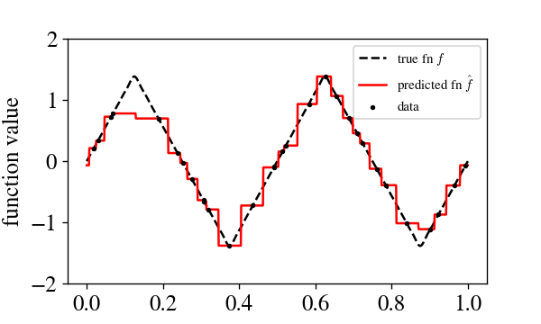
The setting here will be pretty natural: we have some target function $f: [0,1) \rightarrow \mathbb{R}$ we wish to learn, we draw $n$ samples \(\{x_i\}_{i=1}^n\) from $U[0,1)$ and obtain noisy function evaluations $y_i = f(x_i) + \mathcal{N}(0, \epsilon^2)$, and then on each test point $x$ predict $y_{i(x)}$ where $i(x)$ is the index of the closest point to $x$, with circular boundary conditions on the domain. Here’s what it looks like to learn, say, a triangle wave with 20 points:

We will describe generalization in terms of the Fourier decomposition of the target function $f(x) = \sum_{k=-\infty}^{\infty} e^{2 \pi i k x} v_k,$ where ${ v_k }$ are the Fourier coefficients. In terms of the Fourier decomposition, we have that

This is the eigenframework for 1NN in 1D! The generalization of 1NN on any target function in 1D is described by this equation.²

Here are some experiments that show we’ve got it right. The function $\phi_k(x)$ here is the $k$th eigenmode, and we’re using the known Fourier decomposition of the triangle wave.

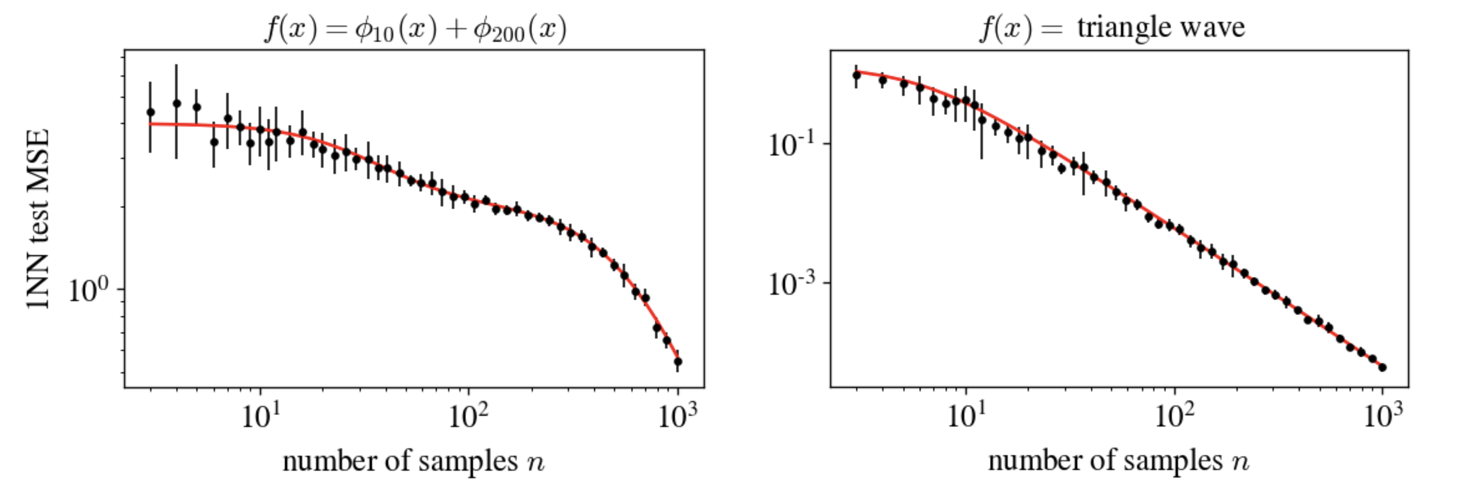
This equation can be found a few ways, but most simply you (a) argue by symmetry that the eigenmodes contribute independently to MSE and then (b) find the test MSE for a particular eigenmode, which isn’t too hard to do. I made two approximations: (1) instead of having exactly $n$ samples, I let the samples be distributed as a Poisson process (i.e., each point has an i.i.d. chance of containing a sample), and (2) I assume the domain is infinite when computing a certain integral. Neither of these matters when $n$ is moderately large.

Before moving on to the 2D case, I want to pause to highlight a few cool features of this framework:

• The Fourier modes do not interact — no crossterms $v_j v_k$ appear in the framework. Because 1NN is a linear learning rule, it’s inevitably possible to “diagonalize” the theory in this way for a particular $n$, but the fact that it’s simultaneously diagonalizable for all $n$ is pretty cool!
• Ignoring the factors of $\pi$, we see that mode $k$ is unlearned when $n \ll k$ and fully learned when $n \gg k$. This makes a lot of sense — it’s sort of a soft version of the Nyquist frequency cutoff.
• Things simplify a bit if, instead of using the index $k$, we write in terms of the Laplacian eigenvalues $\lambda_k = 4 \pi^2 k^2$.

1NN on the 2-Torus

We now undertake the same problem, but we’re in 2D: our data is i.i.d. from $[0,1)^2$, again with circular boundary conditions. Our Fourier decomposition now looks like

\[f(\mathbf{x}) = \sum_{\mathbf{k} \in \mathbb{Z}^2} e^{2 \pi i \, \mathbf{k} \cdot \mathbf{x}}.\]

The same procedure as in the 1D case yields that

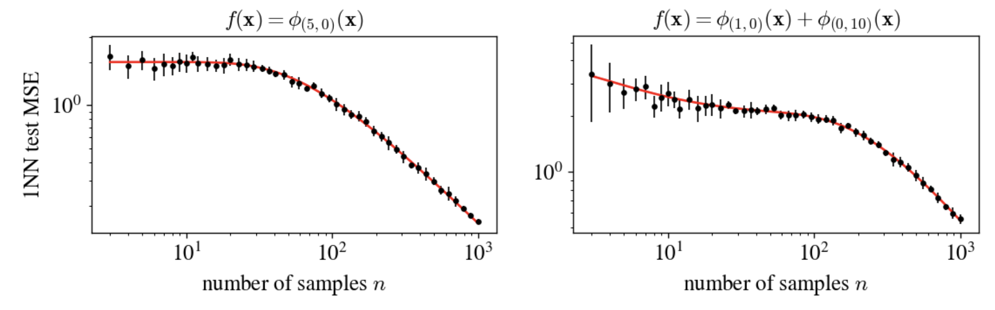
Here are some experiments that show that we’ve got the 2D case right, too.

Can you extend these to k nearest neighbors instead of just one?

Probably! I haven’t tried, though.

Can we find a general theory?

The most remarkable feature of the eigenframework for linear regression is that one set of equations works for every distribution. Can we find that here?

I’m not sure. At first blush, the 1D and 2D equations look pretty different — if we were in search of some master equation, we’d almost certainly want it to unify those two cases, but the functional forms look pretty different! I suspect it might be possible, though — the linear regression eigenframework requires solving an implicit equation that depends on all the eigenvalues and can yield pretty different-looking final expressions for different spectra, so it’s believable to me that there’s some common thread here.

A big question in the search for a general eigenframework is: what’s the right notion of eigenfunction? In these highly symmetric domains, it’s easy — the Fourier modes are the eigenfunctions of any translation-invariant operator we might choose. In general, though, I don’t know what operator we want to diagonalize, or how to use its eigenvalues. This puzzles me. I don’t know the answer! So strange.

Even without a general theory, though, I think it’d be really interesting just to continue this chain of special cases up to the arbitrary $d$-torus! I got stuck at $d=2,$ but I’d bet it can be done. Then we could think about how 1NN differs from kernel regression in high dimensions!³ My understanding is that 1NN is worse, but I don’t actually know any quantification of this. (If you know one, drop me a line!)

So that’s where things stand: these two special cases serve as proof of principle that there might be a general eigenframework for 1NN… and if that exists, it’d be a cool proof of principle that more learning rules than linear regression can be “solved.” Seems like a neat problem! If I make much more progress on it, maybe I’ll write up a little paper. Let me know if you have thoughts or want to collaborate.

---